
Learn how to compare two columns in Excel to find, highlight, or extract matches and differences using various methods.
Sometimes, comparing data can be challenging if you want to use the most effective way. The chosen solution depends on user requirements and the initial data structure.
In this tutorial, you’ll discover several ways to compare two columns in Excel and highlight the matches and differences between them. For example, you can apply conditional formatting to highlight all the matching data points in two columns. As an alternative, use formulas to find matches. We will also demonstrate a custom VBA function to check the similarity between two lists. Last, please take a closer look at our free add-in and learn how to perform all comparison tasks fast.
Table of contents:
- Compare two columns in Excel row-by-row
- Compare two columns and highlight matches and differences
- Find and extract matches between two columns
- Compare two columns and extract differences
- Compare two columns using an Excel add-in
How to compare two columns in Excel row-by-row
Let us start to compare two columns in Excel with some detailed examples. This section will show you how to compare and identify which rows contain the same value and which ones are different.
Compare columns row by row using the equal sign
In the picture below, here is the initial data set. We will compare the names row by row without using built-in Excel functions.
Take a look at the first name in column B. We try to compare the text string with the corresponding item located in the same row, column C. Instead of using a formula; you can perform the comparison with a simple equal sign. The expression gets the result quickly.
=B3=C3The result is a boolean data type; in case of a match, the result is TRUE, else FALSE.
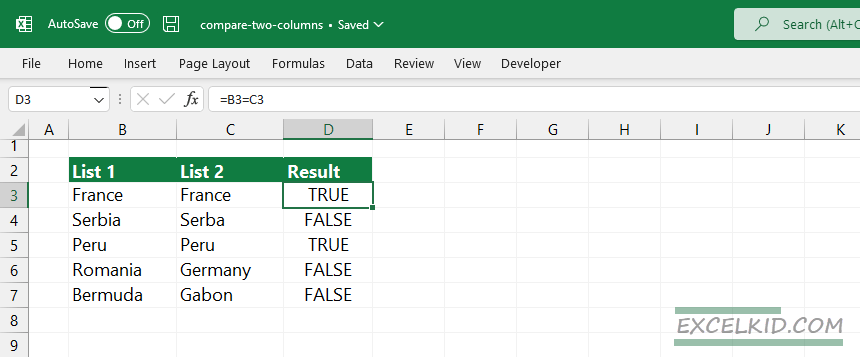
If cell B3 equals C3, Excel will write a TRUE string into column D. Copy the formula down!
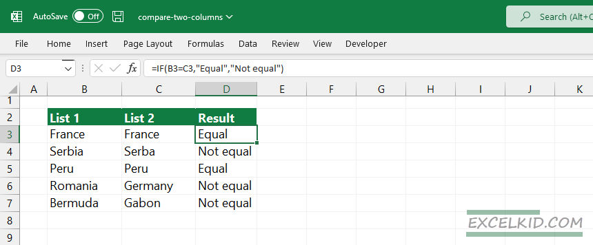
Use the IF function to compare two columns row by row
In the following example, we will make the output easy to read. Choose “Equal” as a second argument and “Not Equal” as the third argument of the IF function; the result will speak for itself. The IF formula returns “Equal” if the given column contains the same name. The result is “Not equal” in case the words are different.
Formula:
=IF(B3=C3,"Equal","Not equal")Result:
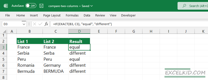
Case-sensitive cell comparison using the EXACT function
In the example, we will use the IF and EXACT functions to find matches to perform case-sensitive cell comparisons. For example, “BERMUDA” and “Bermuda” are not equal; the EXACT function will identify and return a “Not equal” result.
Formula:
=IF(EXACT(B3, C3), "equal", "different")Result:
Compare two columns and highlight matches and differences
Sometimes, we need to compare two columns and highlight matching data. In this example, we will show you how to find duplicates using conditional formatting.
Note: This method is not a row-by-row comparison!
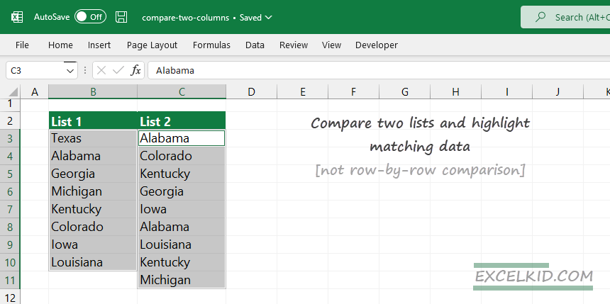
Compare two lists and highlight matching data
The image below shows that the B3:B10 range is not equal to the C3:C11 range. So, at first look, we have matching names but not in the same position.
Follow the steps below to compare two columns with different sizes.
1. Select the range that contains names.
2. Go to the Home tab and choose the Styles group. Click on the Conditional formatting icon.
3. Select the Highlight cell Rules option, then click on the Duplicate values.
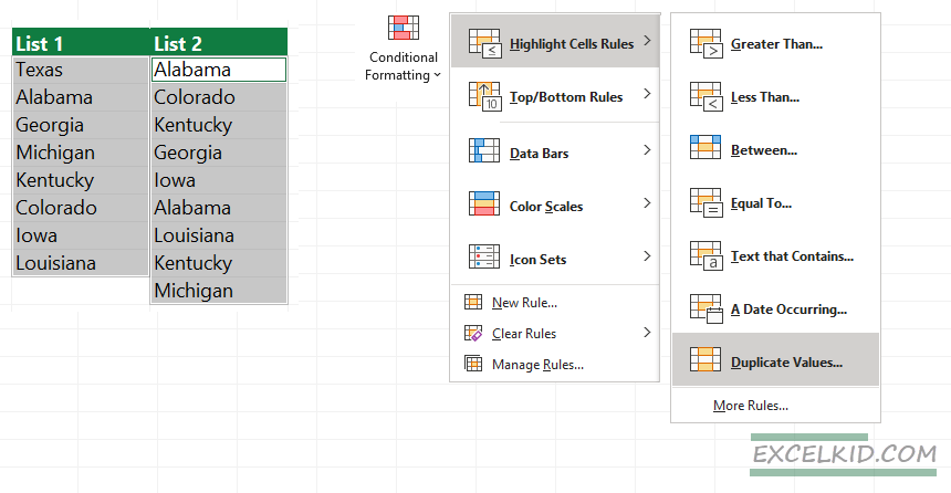
4. The Duplicate Values dialog box will appear. Choose the Duplicate option on the left side of the window.
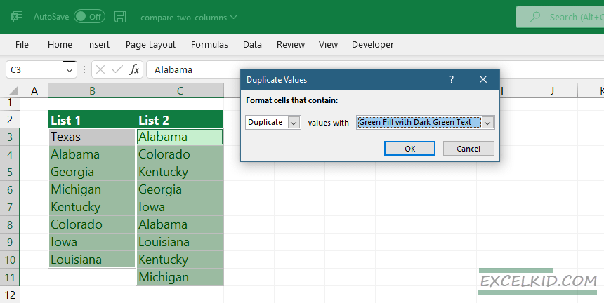
5. Apply your favorite style using the drop-down list, then click OK.
The only non-matching value in this example is Texas in the first list.
Note: This rule is not case-sensitive! “Florida” and “FLORIDA” will be identified as the same and marked as duplicated items.
How to highlight matching data using conditional formatting
How to highlight the same rows in place? The best space-saving solution to do that is using conditional formatting. Excel will highlight the matching cells instead of creating an additional column.
Here are the steps to compare two columns and highlight matches:
- First, select the range which contains the data set.
- Next, click the Home tab on the ribbon.
- Choose the Styles group. Click on the “Conditional Formatting” icon.
- Click on the “New rule” from the drop-down list.
- Locate the “New Formatting Rule” dialog box and click “Use a formula to determine which cells to format.”
- Enter the formula =$B3=$C3 into the formula field.
- Click the Format button to select the format we want to use for the matching cells.
- Click the OK button.
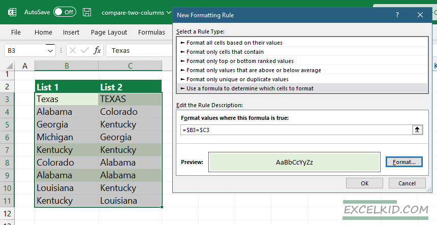
Excel will highlight all the cells where names are equal in each row.
How to compare two columns and highlight unique items
We want to apply an inverse selection to find and highlight unique items in the example.
- Select the range that contains two columns.
- Click the Home tab on the ribbon.
- Navigate to the Styles group and click on the “Conditional Formatting” icon.
- Select the “Highlight Cell Rules” option. Now click on “Duplicate Values“.
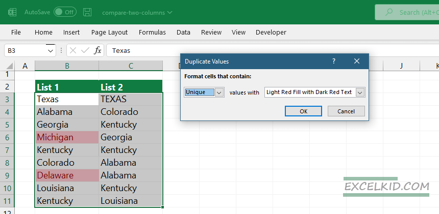
- In the dialog box, select the ‘Unique’ option.
- Set up the styles for cell formatting.
- Click OK.
As a result of inverse selection, Excel will highlight all cells with a unique name that do not exist on the second list.
Find and Extract Matches between two columns
This part of the tutorial will use lookup formulas to compare two lists to find matches.
Exact Data Match: VLOOKUP, INDEX, and MATCH
For example, we want to pull the sales data for List2 based on List1. To do this, use a simple lookup formula.
=VLOOKUP(E3,$B$3:$C$9,2,0)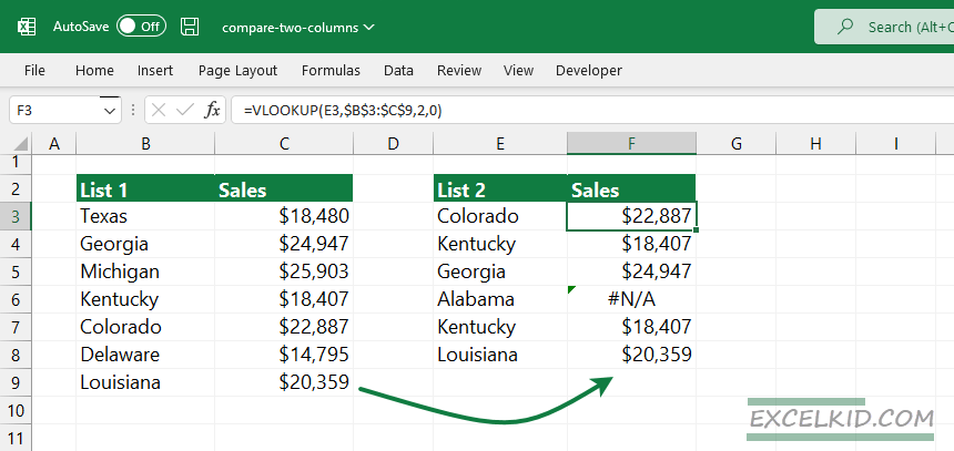
The VLOOKUP function checks whether a record in column B is present in column E or not. If we find a match, the formula will return the corresponding value from column Sales. If the result is different, we get a #N/A error. For example, the formula compares two columns and returns an #N/A error in the case of Alabama since Alabama is not present in the first list.
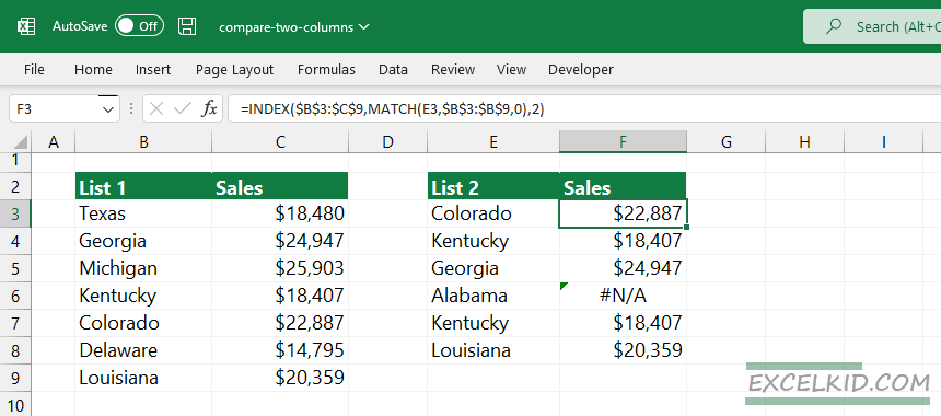
Alternatively, we can use a nested formula containing INDEX and MATCH. We will get the same result as the previously described solution with the VLOOUKUP formula.
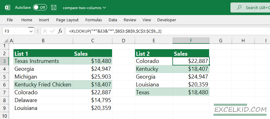
Find a partial match using XLOOKUP
This tutorial will show you the steps of finding partial matches using wildcards by comparing data using two columns. First, use the XLOOKUP function to find a partial match and apply wildcards (asterisk) “*” in Excel.
Using similarity by comparing data in two columns
In this example, we will show you how to calculate the similarity between two strings. We want to consider using a function that will tell us exactly how close two strings are. If you are working on a data cleansing project in Excel, we strongly recommend using it.
If you want to compare two columns that contain similar text strings, is there a way to get the similarity percentage between the two cells in the same row?
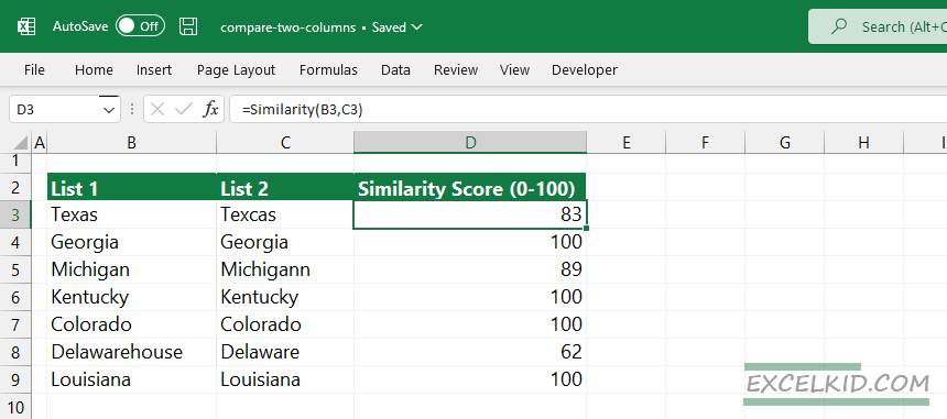
Use the Alt + F11 keyboard shortcut, insert the following code into a new module, or download the practice file. The algorithm tries to find the matching and non-matching parts of the strings and factor them to generate the similarity score. The result is an integer between 0 and 100.
Function Similarity(ByVal str1 As String, ByVal str2 As String) As Long

Dim i As Long, j As Long, str1_length As Long, str2_length As Long
Dim gap(0 To 60, 0 To 50) As Long, sm1(1 To 60) As Long, sm2(1 To 50) As Long
Dim m1 As Long, m2 As Long, m3 As Long, mm As Long, MaxL As Long

str1_length = Len(str1):  str2_length = Len(str2)

gap(0, 0) = 0
For i = 1 To str1_length:    gap(i, 0) = i: sm1(i) = Asc(LCase(Mid$(str1, i, 1))): Next
For j = 1 To str2_length:    gap(0, j) = j: sm2(j) = Asc(LCase(Mid$(str2, j, 1))): Next
For i = 1 To str1_length
    For j = 1 To str2_length
        If sm1(i) = sm2(j) Then
            gap(i, j) = gap(i - 1, j - 1)
        Else
            m1 = gap(i - 1, j) + 1
            m2 = gap(i, j - 1) + 1
            m3 = gap(i - 1, j - 1) + 1
            If m2 < m1 Then
                If m2 < m3 Then mm = m2 Else mm = m3
            Else
                If m1 < m3 Then mm = m1 Else mm = m3
            End If
            gap(i, j) = mm
        End If
    Next
Next

MaxL = str1_length: If str2_length > MaxL Then MaxL = str2_length
Similarity = 100 - CLng((gap(str1_length, str2_length) * 100) / MaxL)

End Function
Compare Two Columns and Extract Differences
This section will show you some atypical methods to compare two columns and extract the result into a new list.
FILTER formula to compare unsorted lists (Excel for Microsoft 365)
This section will show you formulas that extract values that exist only in one column out of two columns. The solution uses the FILTER and COUNTIF functions to extract differences. Don’t forget to update your Excel if you want to use the FILTER function; it’s available from Excel 2019.
=FILTER(C3:C9,COUNTIF(B3:B9,C3:C9)=0)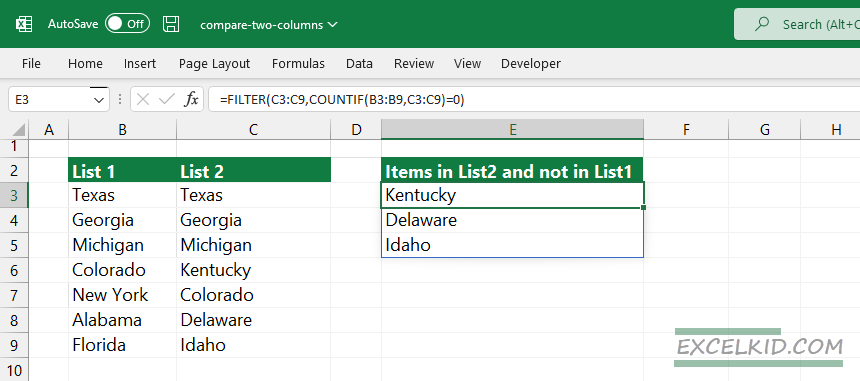
The formula in cell E3 extracts values in cell range C3:C9 that are not in cell range B3:B9. So we find the records; they exist only in cell range B3:B9. For example, the value “Kentucky” in cell C6 is not in range B3:B9; however, the value “Texas” in cell C2 also exists in cell range B3:B9, in cell B3.
Now, we want to extract differences using the following rule: Extract items that exist in List 1 and not exists in List 2.
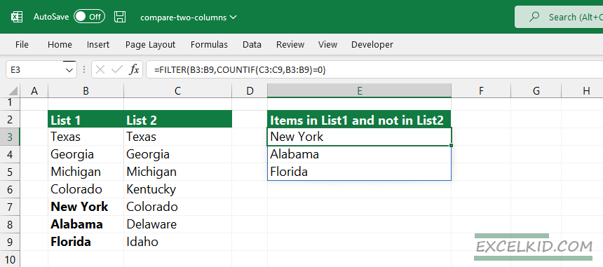
Formula:
=FILTER(B3:B9,COUNTIF(C3:C9,B3:B9)=0)Compare two columns using sorted elements (older Excel versions)
Use the following workaround if you have an older version of Microsoft Excel (Excel 2013 or Excel 2016).
Apply the following formula in cell E3. Press Ctrl + Shift + Enter instead of using a simple Enter.
=INDEX($B$3:$B$9, SMALL(IF(COUNTIF($C$3:$C$9, $B$3:$B$9)=0, MATCH(ROW($B$3:$B$9), ROW($B$3:$B$9)), ""), ROWS($A$1:A1)))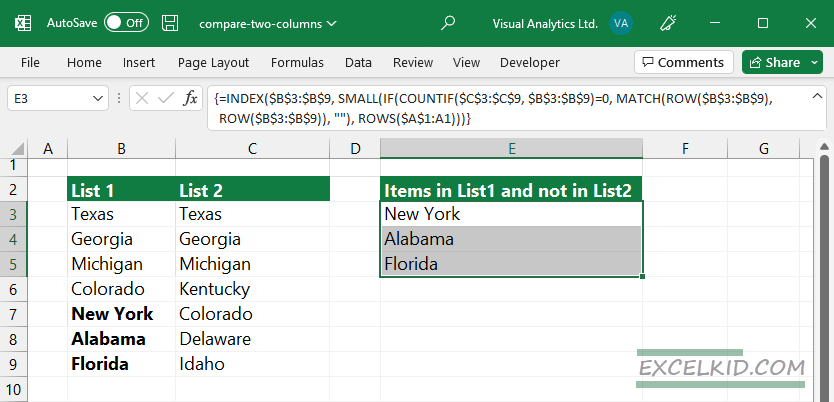
How does the formula work?
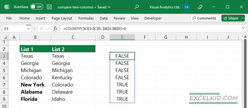
The expression below counts values in List 1 based on values in List 1.
=COUNTIF($C$3:$C$9, $B$3:$B$9)=0The result is an array that contains TRUE and FALSE values:
To replace TRUE with the corresponding row number, use:
=(IF(COUNTIF($C$3:$C$9,$B$3:$B$9)=0,MATCH(ROW($B$3:$B$9),ROW($B$3:$B$9))))For example, if we want to find the n-th smallest row number, apply this formula below:
=SMALL(IF(COUNTIF($C$3:$C$9,$B$3:$B$9)=0,MATCH(ROW($B$3:$B$9),ROW($B$3:$B$9)),""),ROWS($A$1:A1))Finally, you must extract the list’s 5th, 6th, and 7th items. The result array contains New York, Alabama, and Florida.
Compare two columns using an Excel add-in
Everyone knows that VBA is a powerful programming language. Add-ins, macros, or custom (user-defined) functions are worth using to perform string manipulations. All you need is logical thinking to automate your tasks. Your daily work will be easier, guaranteed.
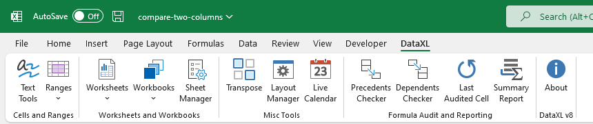
The following examples show you how to compare two columns and extract matches and differences without formulas. But first, install our free Excel add-in, DataXL. After the successful installation, you will see the DataXL tab on the ribbon.
Our goal is to make advanced methods more straightforward and transparent. Sometimes, you can use Excel automation instead of boring formulas and functions.
Extract the records from a range that coincides with another range
Steps to extract matches and differences from two lists:
1. Go to the ribbon, locate the DataXL tab, and select the Ranges icon.
2. From the drop-down list, choose the Compare Ranges function
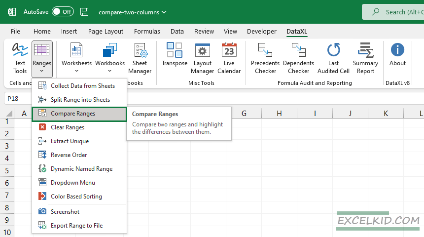
3. The Compare ranges dialogue box will appear after clicking the icon.
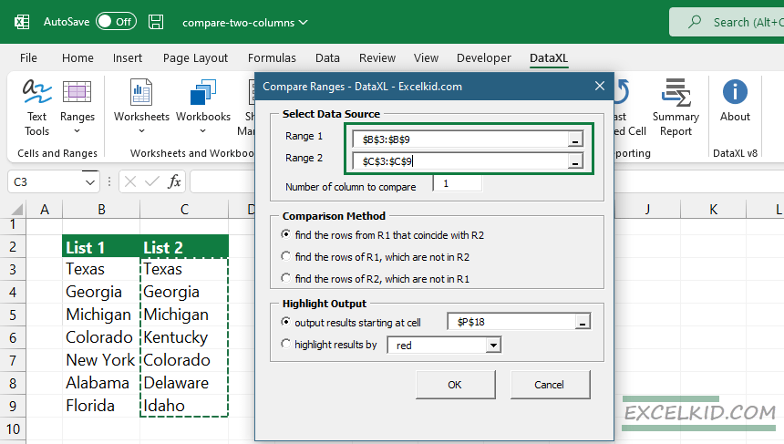
4. Select the data sources
5. Under the Comparison Methods tab, choose Option 1
6. Select the output cell
7. Finally, Click OK
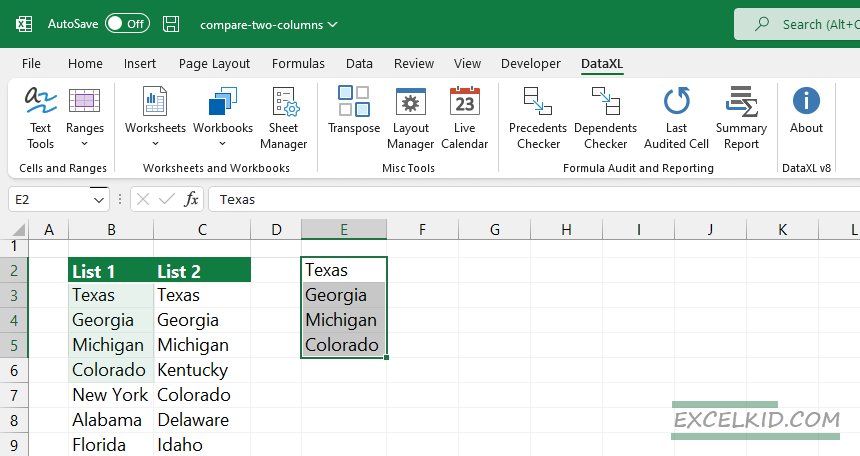
You can use the add-in to compare two tables, ranges, or lists. The tool supports two output types; use the first option (“Output results starting at cell….”) to extract the matching items in a new place. Apply the second option to compare and highlight the matching records using the selected font color in place.
We hope you enjoyed our definitive guide! Stay tuned.