Highlight Every Other Row in Excel

This tutorial will explain how to highlight every other row in Excel. Then, to improve your spreadsheet’s readability, alternate shade rows!

Working with large data tables and organizing ranges in Excel is sometimes not too easy. In this Excel guide, I will cover the following topics:

At first, you’ll learn how to highlight every other row using conditional formatting. After that, we’ll introduce the excel-table based solution. Finally, we’ll write a short macro to get the work even faster for shading every other row.

How to highlight every other row in Excel using Conditional Formatting

Frequently facing the problem: It would be great to highlight rows in Excel! Conditional formatting is a versatile tool for highlighting rows, columns, and values colors, so we’ll use it in this example.

Shade alternate rows using the ISEVEN function

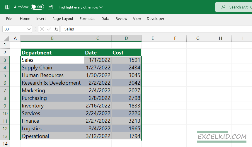
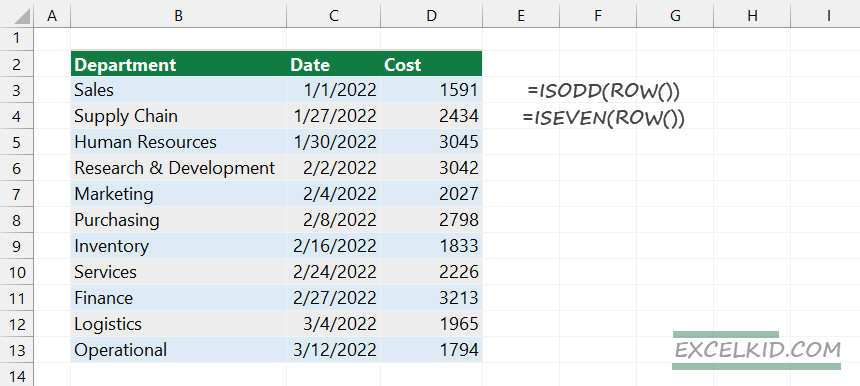
We shade every other row in the B3: D13 range in this example. To quickly highlight every alternate row in Excel, follow the steps below:

1. Select the range which contains data

2. Save your time using keyboard shortcuts! Use the Alt + O + D shortcut to open the conditional formatting rules manager window.

3. If you are unfamiliar with Excel shortcuts, click on the Home tab, select Conditional Formatting, and choose New Rule.

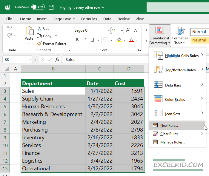
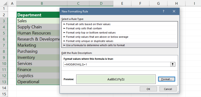
4. Apply a custom formula! First, select the “Use a Formula to determine which cells to format” option in the “New Formatting Rule” dialogue box.

5. Now, apply the formula to a range of cells. Select the “Edit the Rule Description” field, and type the formula:

=ISEVEN(ROW())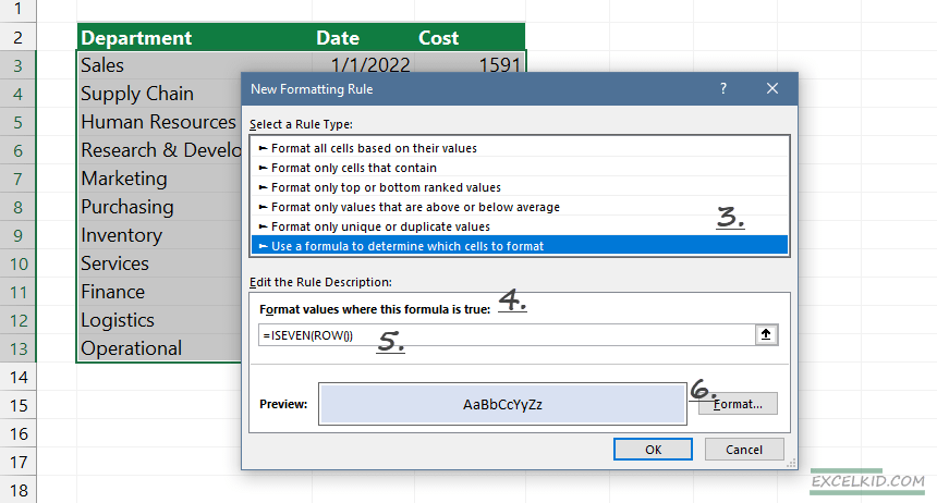

6. Click on the Format button and choose the fill color.

7. Click OK to highlight alternate rows.

Combine ISEVEN and ISODD functions to apply unique Zebra Stripes

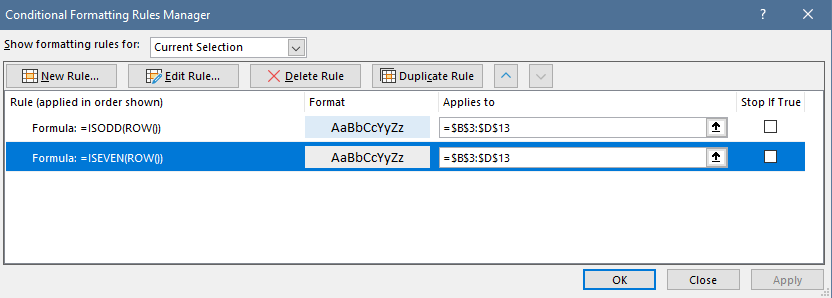
To create unique row styles, combine the ISEVEN and ISODD functions. Add a second rule to Conditional Formatting Rules Manager.

Formula:

=ISODD(ROW())

Apply the ISODD and ROW combination. The result of the formula will be TRUE if the row number is odd. Otherwise, you’ll get FALSE as a result of the expression.

Explanation: If you run a nested formula using ISEVEN and ROW, the expression will return TRUE if the number is even. The result will be FALSE if the row number is odd. This method highlights the 1st, 3rd, 5th, (and so on) row in a range.

Highlight every other row using the MOD function

You can use the MOD function if you are working with rows and colors. Go to the Rules Manager and replace the formulas with a new ones. The formula is the following:

=MOD(ROW(),2)=1

You can apply the combination of MOD and ROW functions to create a custom formula and get the remainder from the division.

Evaluate the formula! Because the ROW function returns 3;

=MOD(ROW()),2)=1

Excel will compile the formula into the following:

=MOD(3,2) = 1

As a result of the formula, Excel highlights the first row because the result meets our initial criteria. Now use the formula for the next row! The =MOD(4,2) expression will get 0, so it does not meet our criteria, and the row remains unchanged.

Shading every nth row or column

Sometimes you want to highlight every nth row, for example, every 5th row. Then, if you change the parameters of the ROW formula, you can work without limits.

Examples to highlight every nth row:

=MOD(ROW(),4)=1 //shade every 4th row
=MOD(ROW(),5)=1 //shade every 5th row

Formatting Excel Tables for highlighting rows

If you are working with Excel tables, let us see the lightspeed solution for shading every other row.

Example 1: Using built-in table styles

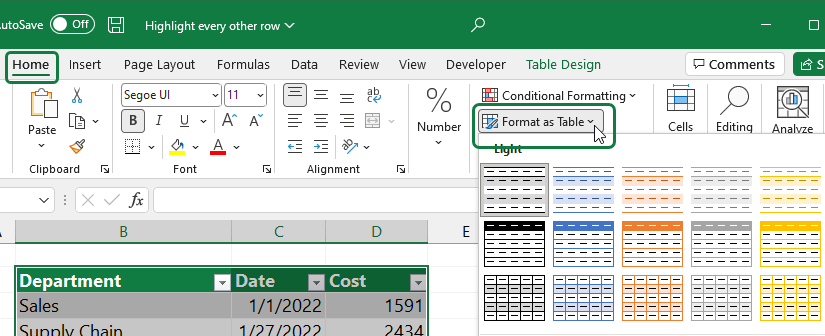
1. Select the range which contains data.
2. Choose the Home tab and click on the Format as Table
3. Click on the predefined styles window and choose one of them.

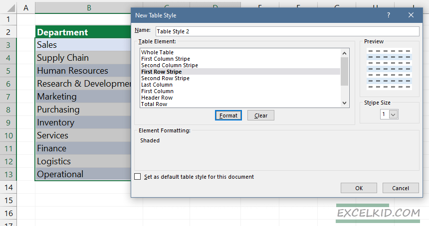
Example 2: Create your custom style for alternate shading rows

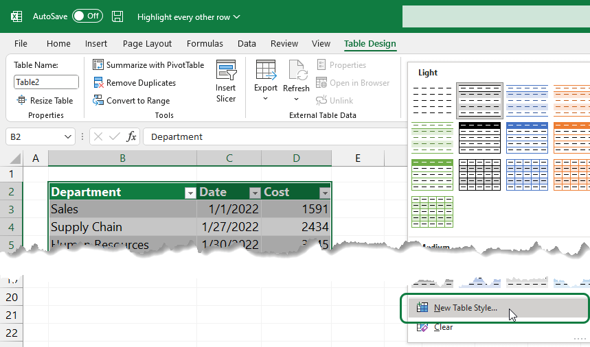
Select the table, and click on the Table Design Tab.

Steps to create stripes:

1. Click on the ‘New Table Style.’
2. Then, select ‘First Row Stripe’ in the New Table Style dialogue box.
3. Click Format and select the color for shading. The preview window will show your chosen color scheme. To apply this style frequently, click on ‘Set as default table style for this document‘.
4. Click OK.

VBA macro to Highlight Every Other Row in Excel

To insert a macro open Visual Basic Editor on the Developer tab and click Visual Basic.

Suppose you prefer keyboard shortcuts; press Alt + F11 to open the VBE window.

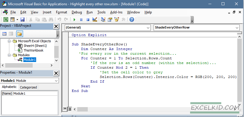
1. Right-click on the workbook name.
2. Select Insert -> Module from the context menu.
3. Copy and paste the code to the right pane.

Sub ShadeEveryOtherRow()
    Dim Counter As Integer
   'For every row in the current selection...
    For Counter = 1 To Selection.Rows.Count
        'If the row is an odd number (within the selection)...
        If Counter Mod 2 = 1 Then
            'Set the cell color to grey
            Selection.Rows(Counter).Interior.Color = RGB(200, 200, 200)
        End If
    Next
End Sub

To start the macro, follow these steps:

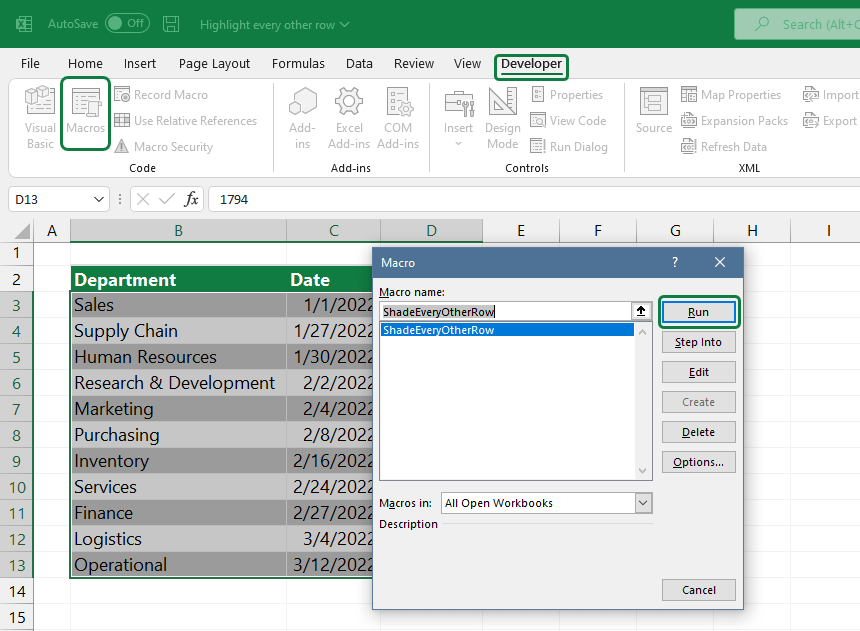
1. Go to Developer Tab (if it does not appear, enable it)
2. Click Macros
3. The Macro dialogue box appears.
4. Select the macro and click Run.

Download the sample Workbook.

Additional resources

• Compare two columns in Excel