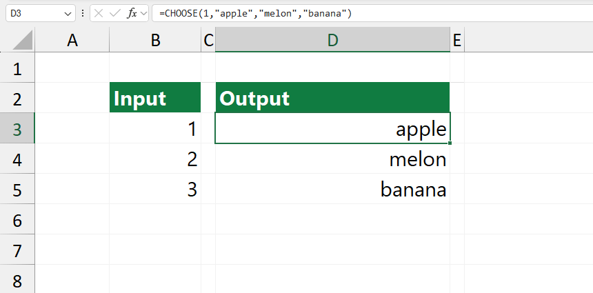
The Excel CHOOSE function allows you to select a value from a larger set of options by adding an index of the value you want to retrieve.
For example, the =CHOOSE(3,”apple”,”melon”,”banana”) will return “banana”, since banana is the 3rd value listed based on the index number. There are two restrictions: You can use only positive integer values as a first argument. Furthermore, the CHOOSE function supports selecting values (index numbers) between 1 and 254.
How to use the CHOOSE function in Excel
Syntax.
The function uses the following syntax:
=CHOOSE (index_num, value1, [value2], …)
Arguments
The function uses at least two required and optional arguments:
- index_num – The selected value, index_num, should be between 1 and 254.
- value1 – The first variable in the list you can choose.
- value2 – [optional] The second value to select.
Examples
In the example, use the following formulas to return the first, second, and third values from a predefined list:
=CHOOSE(1, “apple”, “melon”, “banana”, “lemon”) //returns “apple”
=CHOOSE(2, “apple”, “melon”, “banana”, “lemon”) //returns “melon”
=CHOOSE(3, “apple”, “melon”, “banana”, “lemon”) //returns “lemon”
The function cannot manage ranges. If you add a range as a second parameter, Excel will return a #VALUE error.
=CHOOSE(3,B1:B3) = #VALUE
The formula returns error, because the proper syntax is =CHOOSE(3,B1, B2, B3)
CHOOSE works great if the list is short. However, if you have a large data set, we recommend using the much faster and more versatile XLOOKUP function to get the selected value based on a position.
=XLOOKUP(300,A1:A300,B1:B300) will return the 300. record from column B.
Don’t forget the most important disadvantages of using the CHOOSE function: You have to use hardcoded values, like {“apple”, ”banana”, ”melon”}. You can manually fill the array using text values to shorten the formula.
Workaround CHOOSEROWS Function
The CHOOSEROWS function, available in newer Excel versions, simplifies selecting specific rows from a range. Instead of manually listing items, CHOOSEROWS allows you to reference a range and specify which row(s) you want to extract.
The example =CHOOSEROWS(C3:C5, 3) returns the value “banana” because it selects the 3rd row from the range C3:C5.
Advantages of CHOOSEROWS over CHOOSE:
- CHOOSEROWS can operate on ranges, making it easier to adapt to data changes. If the values in C3:C5 change, it automatically reflects those changes, while CHOOSE requires manual adjustments.
- With CHOOSEROWS, you can avoid manually entering each item, which is especially useful in larger datasets.
- The formula is easier to read since it directly references the range instead of listing individual items.
Formula examples:
=CHOOSE(3, “apple”, “melon”, “banana”) = banana
=CHOOSEROWS(C3:C5, 3) = banana
The result is the same, but the formula is simple.