XLOOKUP Function in Excel

Use the XLOOKUP function in Excel to handle vertical or horizontal arrays and support the exact match, wildcards, and binary search.

We are happy to provide this comprehensive guide about the XLOOKUP function in Excel. Generally, the function has changed everything in Excel in the last few years. We built the tutorial from the ground up. First, we overview how the XLOOKUP function works in Excel. Next, the second part of our step-by-step guide provides practical, detailed examples. Finally, you can learn how to fix your formulas if the function is not working properly.

To reduce your learning curve, use the Workbook that contains all examples.

Download the practice file.

Table of contents:

• What is XLOOKUP?
• How can I get XLOOKUP?
• How to use XLOOKUP Function?
  • Exact match: How the left lookup works
  • Error handling: The “if not found” argument
• XLOOKUP Match mode
  • Find the next smaller item (closest value)
  • Find the next larger item (closest value)
  • Partial match (wildcards)
• XLOOKUP search mode
  • Search in reverse order to get the last occurrence
  • First to last search mode
  • Binary search
• XLOOKUP Function and Formula Examples
  • Return All Matches
  • SUM multiple rows based on a lookup value
  • Using a two-way lookup
  • XLOOKUP match text contains
  • Lookup value between two numbers
  • Using logical criteria
  • Using multiple criteria
  • Lookup row or column
  • XLOOKUP with boolean or logic
  • XLOOKUP across multiple Worksheets
  • Find the 2nd or nth match
  • Get the first text value
  • Find the first or last positive value in a list
  • XLOOKUP return blank if blank
  • Case sensitive lookup
• XLOOKUP vs. VLOOKUP
• Why is XLOOKUP not working properly?

What is XLOOKUP?

XLOOKUP provides never seen before flexibility for Excel. You can use it instead of older lookup functions like VLOOKUP or HLOOKUP. Another good news is that no INDEX + MATCH workaround is necessary.

How can I get XLOOKUP? (all Excel versions)

XLOOKUP is available for Microsoft 365 users by default. However, installing a small add-in can use the function with other Microsoft Excel (2010, 2013, 2016, 2019) versions.

Steps to add XLOOKUP function for Excel 2013, 2016, and 2019:

1. Open Excel
2. On the Developer Tab, click Excel Add-ins
3. Click Browse and select the DataFX add-in
4. Click OK
5. The function is ready to use

You can learn more about the project here.

How to use XLOOKUP Function

In this part of the tutorial, first, we will explain the basics. You will learn how the two main parts of the function work. Let us see the syntax and arguments!

Syntax, Arguments

XLOOKUP uses a similar syntax as VLOOKUP but provides some improvements, like the error-handling argument.

=XLOOKUP(lookup value, lookup array, return array, [if not found], [match mode], [search mode])

The function uses six arguments: three required and three optional.

Required arguments:

• Lookup value: the value you are looking for in the lookup array
• Lookup array: the range where you find the lookup value
• Return array: the range which you want to result

Optional arguments:

• If not found: error handling option when the lookup value is not found
• Match mode: Controls the match mode and type
• Search mode:

Exact match: How the left lookup works

In the first example, we use the XLOOKUP left lookup functionality. Please look at how easy it is to replace the VLOOKUP, HLOOKUP, LOOKUP, and the INDEX + MATCH functions. You do not need to apply a 0 for an exact match.

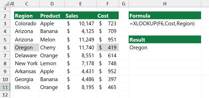
We aim to find the matching value in the Region column where the Cost is $419.

To simplify our task, create named ranges! Select range C3:C11, locate the name box, type ‘Region‘, and press enter.

Define the following named ranges:

• Region: C3:C11
• Product: D3:D11
• Sales: E3:E11
• Cost: F3:F11

The following formula performs a left lookup:

=XLOOKUP(F6, Cost, Region)

You can use the VLOOKUP and CHOOSE functions as a workaround for reverse lookup. The CHOOSE function swaps columns and restructures data for VLOOKUP.

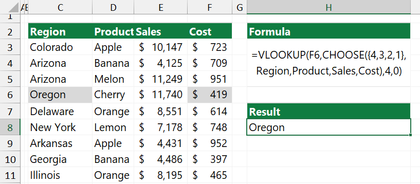
=CHOOSE({4,3,2,1},Region, Product ,Sales, Cost)

LEFT lookup using VLOOKUP:

=VLOOKUP(F6,CHOOSE({4,3,2,1},Region, Product, Sales, Cost),4,0)

Error handling: The “if not found” argument

By default, the XLOOKUP function (like other lookup functions in Excel) returns an #N/A error if it does not find a matching value in the return array. Use the “if not found” optional argument for error-handling purposes.

Instead of using an extra function – like IFNA – you can replace #N/A with a more readable “No matching value” message. This step reduces the length of the formula, which is a great advantage. In the example, we show how to customize the result instead of the default #N/A.

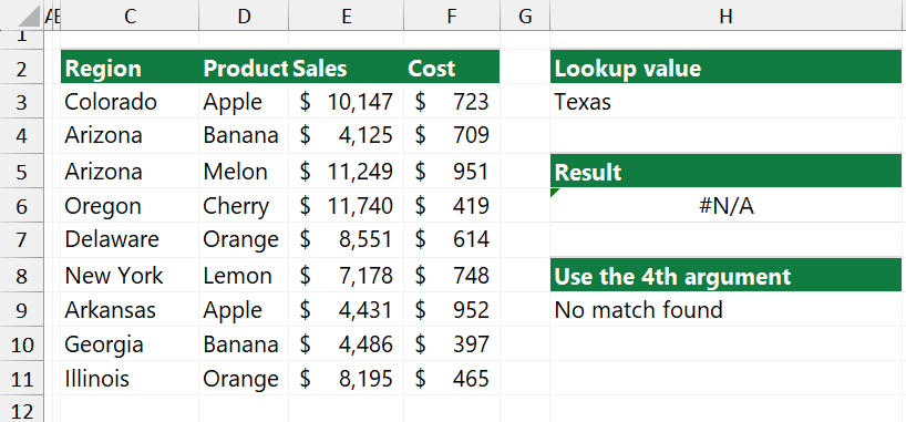
In the example, we want to find Sales where the Region is Texas. The lookup array (column C) does not contain the string “Texas” (lookup value). Without error handling, the formula returns #N/A. Apply the 4th argument.

=XLOOKUP(H3,Region,Sales,"No match found")

The formula handles the #N/A error and returns a custom, user-defined text value, “No match found.”

XLOOKUP Match mode

The match mode is an optional argument to control the types of matches. Here is the list of the values:

• The function uses “0″ by default: an exact match; the function returns #N/A if no match is found.
• To get an exact match or the next smaller item (approximate match), use “-1“.
• To return an exact match or the next smaller item, use “1”.
• For partial or wildcard matches, set the 4th argument to “2”.

This tutorial will explain how to use the match mode argument.

Find the next smaller item (Closest value)

In the first example, we demonstrated how the exact match works. Because the default is 0, you do not need to use the argument. Sometimes, you need to find the closest value, in this case, the next smaller item.

We use the 5th argument to get the second match, smaller than the exact match. We want to find the Region where the lookup value in the Sales column is less than or equal to $8600.

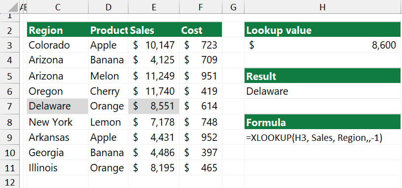
Use the formula below and set the match mode argument to -1:

=XLOOKUP(H3, Sales, Region,,-1)

Explanation: The formula searches for an exact match based on the lookup value of $8600. In the Sales column, there is no exact match found. The formula finds the nearest lookup value in the column. Using an approximate match, the function will use the next smaller item as a lookup value. As you see, $8551 meets the criteria. Finally, the formula returns “Delaware”.

Find the next larger item (Closest value)

Now, try to use an inverse search and find the closest value greater than or equal to the lookup value. The method is the same as the example above. First, we will try to find an exact match. If the value is not found in the lookup array, XLOOKUP takes the next larger value.

We want to find the corresponding Region in the first column based on the lookup value. The table clearly shows that there is no exact match. In this case, the next larger item in the lookup array is 4486.

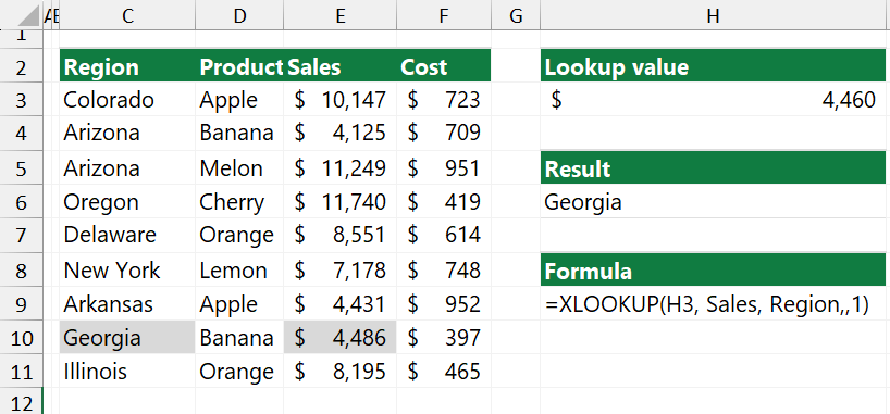
Formula:

=XLOOKUP(H3, Sales, Region,,1)

The formula returns “Georgia”, where the Sales are 4486.

XLOOKUP with partial match (wildcards)

The wildcard character match mode provides a partial search option. In the example, we are looking at the Region that begins with “AR”. Set the match mode to 2 to return the sales based on the lookup value.

• lookup value: = “Ar*”
• lookup array = Region
• return array = Sales
• match mode = 2

Formula:

=XLOOKUP(H3, Region, Sales,,2)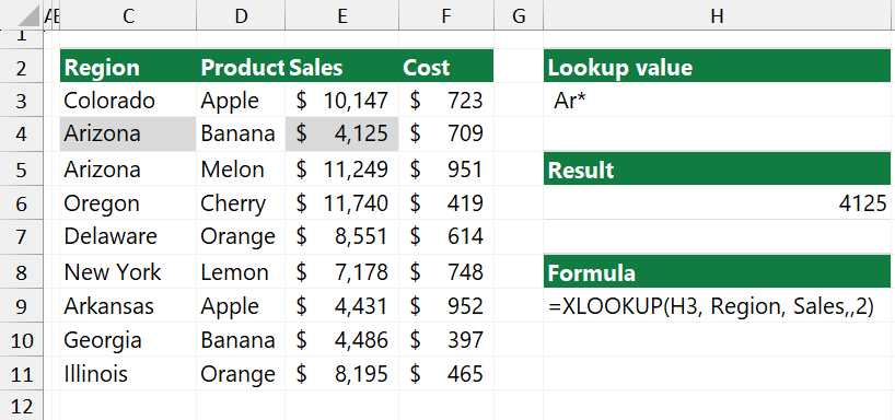

You can use wildcard search in other cases, too. What if you want to replace only a single letter? Use the “?” symbol and set 2 to the 5th argument. You can replace a single letter, but the match mode works fine with multiple letters.

Formula:

=XLOOKUP(H3, Region, Cost,,2)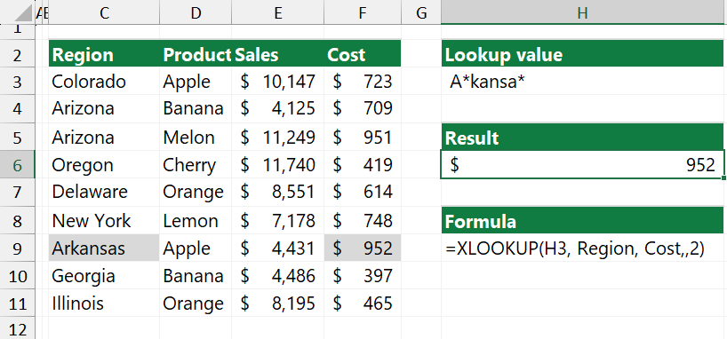

The formula performs a lookup and returns the cost for Arkansas.

XLOOKUP Search mode

By default, the XLOOKUP function gets the first matching value. However, you can configure the 6th argument to apply reverse search mode.

You can use the following options:

• Default search mode = 1
• Search in reverse order = -1
• Binary search: values sorted in ascending order = 2
• Binary search: values sorted in descending order =-2

Search in reverse order to get the last occurrence

In the example, we use -1 (match direction) as the search mode argument to perform a last-to-first search and return the matching value in reverse order. We want to find the sales for Arizona, and the formula gets the last occurrence.

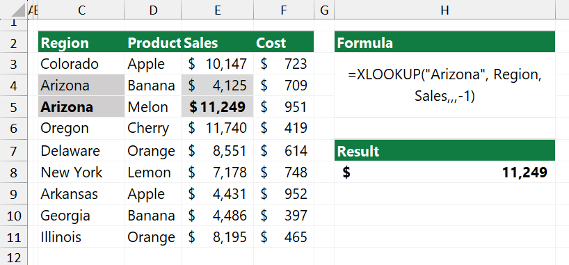
Formula:

=XLOOKUP("Arizona", Region, Sales,,,-1)

Explanation: Look at the comma-separated list inside the formula. We use only the search mode optional argument. To skip an argument, replace it with a comma. The result is $ 11,249 since the function a reverse search. That means it starts with the last match.

XLOOKUP first to last search mode

The default search mode uses the top-to-bottom search. Now, try another formula to get the first matching value. The lookup value is “Arizona”, and the lookup array is the “Region” column.

To perform a first-to-last search, use ‘1‘ as a search mode argument.

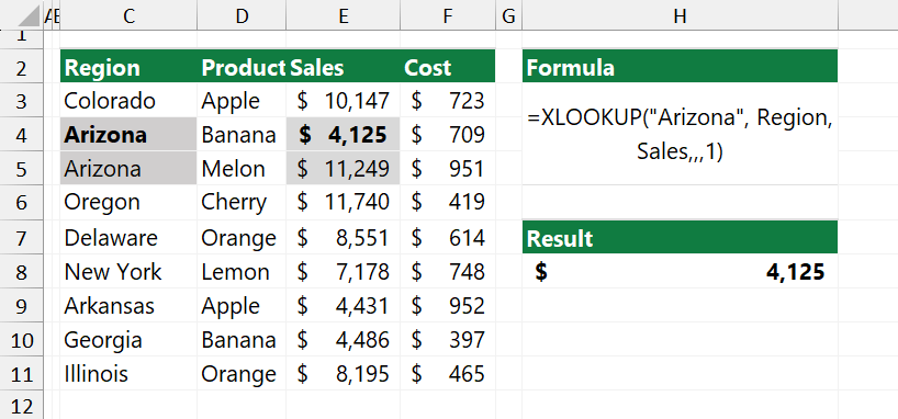
Formula:

=XLOOKUP("Arizona", Region, Sales,,,1)

Explanation: The formula uses a top-to-bottom search. It takes the lookup value “Arizona” and searches for the first matching value in the Sales column. The result is $4125.

Binary search mode

The reason we use binary search is the amount of the data. This search mode can be faster than the default (linear) search mode. Ensure your data is sorted elsewhere. You will get an #N/A error. To perform a binary search, set the search mode argument to 2.

Evaluate the formula:

=XLOOKUP(E11,Sales,Region,,,2)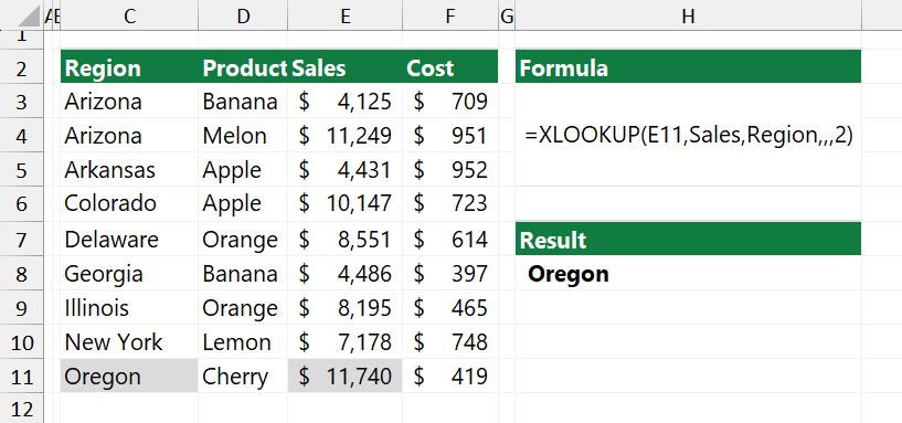

Explanation: In the example, the lookup value is $11,740, and we find the match in the Region column. The data is sorted in ascending order, so we use “2” as a 6th argument. In another case, where the data is sorted in descending order, use “-2“.

XLOOKUP Function and Formula Examples

Now, we have learned the basics. The following section contains various examples from the beginner level to the advanced.

XLOOKUP Formula to Return All Matches

How do I get XLOOKUP to return all matches if it can not provide them? Use a workaround with the FILTER function. It uses two required arguments to return all matches:

Generic formula:

=FILTER(array, include, [if_empty])

First, type the FILTER function. Next, add the first return array argument, range Region. Finally, use a custom criteria (expression) for the second argument.

Configure the arguments:

• “array“: the array where we find the matching records, C3:E11
• “include“: Region=” Arizona“

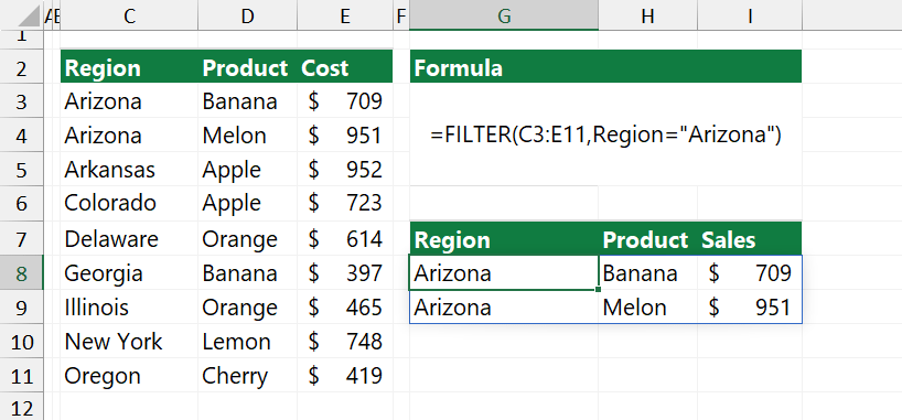
Formula in cell G8:

=FILTER(C3:E11,Region="Arizona")

Explanation: The 2nd argument, [include], finds all matching records from the entire range. The FILTER function returns the matching rows where the Region equals “Arizona”. FILTER is a dynamic array function; Excel spills all records that meet the criteria.

SUM multiple rows based on a lookup value

To sum multiple rows based on a lookup value, you can use XLOOKUP instead of VLOOKUP. A simple vertical lookup finds and summarizes the matching records in the given row.

The SUM function creates an array and then summarizes the matching values. Finally, it returns the result into a single cell.

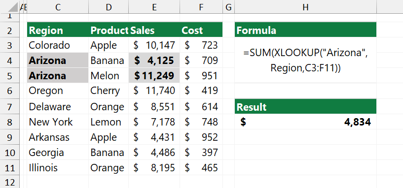
Formula:

=SUM(XLOOKUP("Arizona", Region,C3:F11))

Nested XLOOKUP: Using a two-way lookup

Let us see how a nested XLOOKUP formula works. We use two lookup values in the example to find the matching values. The reason is to replace and simplify the INDEX and MATCH methods. The two-way lookup returns an exact match, but you can use two criteria.

In the example, we want to find sales where the Period is Q4, and the Region is New York.

Named ranges:

• Region: C3:C7
• Period: D2:G2
• Sales: D3:G7

Formula:

=XLOOKUP(J3,Period,XLOOKUP(J2,Region,Sales))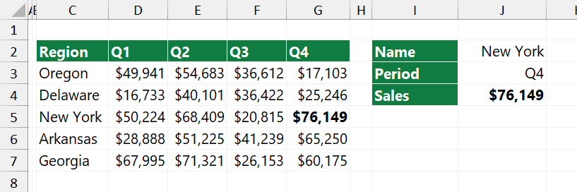

Explanation: The inner lookup formula returns an array where we will find the Sales. The outer formula uses the array as a lookup array. The matching value is Q4, so the formula returns the 4th value in a Sales range.

=XLOOKUP(J3, Period, {50224, 68409, 20815, 76149})

XLOOKUP match text contains

To find text matching text values, use the wildcard character match mode. As you know, XLOOKUP has wildcard support by default. If you want to match text containing one or more characters, use “2” as a 6th argument. In this case, we leave the first to last search mode.

The lookup value is “BS“. Let us try to find the price in the second column. First, construct the lookup value: concatenate the text with two wildcards (*).

“*” & BS & “*”

This part of the formula finds a partial match in the ID column.

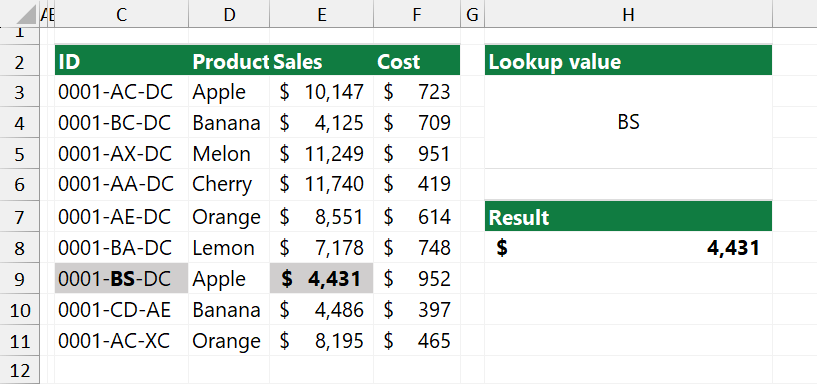
The result is $4,431 since we have a partial match in row 9.

Formula:

=XLOOKUP("*BS*", ID, Sales,,2)

Note: ID and Sales are named ranges.

Lookup value between two numbers

To find values between two numbers, you can use XLOOKUP. The match mode argument provides approximate matches if no exact match is found. In this case, the result is the next smaller item.

To create a better formula, we use named ranges:

• Low = F3:F9
• Rating: G3:G9

=XLOOKUP(C3,Low,Rating,,-1)

Set up the arguments:

• lookup value = C3
• lookup array = “Low” (F3:F10)
• return array = “Rating” (H3:H10)
• match mode = -1

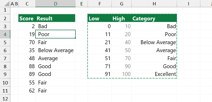
Explanation: The formula finds an exact match in the Score column and gets the corresponding value from the “Rating” range. Finally, it returns the next smaller item if no exact match is found.

XLOOKUP with logical criteria

In the example, we want to find the Region that meets the following requirements:

• The product is equal to “Banana”
• Sales are greater than 4200

Type the formula in cell H8:

=XLOOKUP(1,(Product="Banana")*(Sales>4200),Region)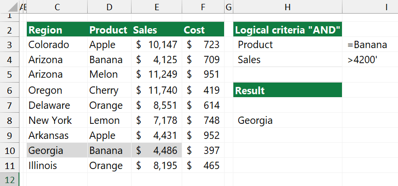

The formula returns the first Region, where the Product = “Banana” AND the sales exceed 4200.

Explanation: We construct a lookup array using boolean logic. Excel returns two arrays containing TRUE or FALSE values to calculate the product of two arrays.

The result of the Product array:

={FALSE, TRUE, FALSE, FALSE, FALSE, FALSE, FALSE, TRUE, FALSE}

The result of the Sales array:

={TRUE, FALSE, TRUE, TRUE, TRUE, TRUE, TRUE, TRUE, TRUE}

The final array contains 0 or 1 values:

={0;0;0;0;0;0;0;0;1;0}

The formula finds the first match in row 8 and returns “Georgia“

XLOOKUP with multiple criteria

This tutorial explains how to use the XLOOKUP function with multiple criteria. We will construct the lookup value in the example by concatenating the arguments. To create a single lookup value from the multiple criteria, we use the “&” sign.

We want to find the Sales where the:

• Region = “Arizona”
• Product = “Melon”
• Quality = “Excellent”

The generic formula looks like this:

=XLOOKUP(criteria1&criteria2&criteria3, range1&range2&range3, results)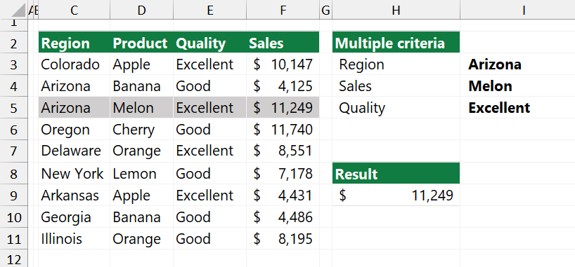

Configure the arguments:

• lookup value: I3&I4&I5
• lookup_array: Region&Product&Quality
• return_array: Sales

In the example, the formula in H9:

=XLOOKUP(I3&I4&I5, Region&Product&Quality, Sales)

The formula returns $11,249, the sales for excellent quality melon in Arizona.

Lookup row or column

The following example will show you how to perform a row or column lookup using XLOOKUP instead of the INDEX and MATCH functions. We aim to return an entire row or column using a single function.

In the example, we want to return all Sales for March”, so we use the function to look up a column. For the sake of simplicity, we use the following named ranges:

• Months
• Data

Formula:

=XLOOKUP(H2,Months, Data)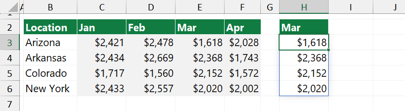

Let us evaluate the formula. First, the formula finds the lookup value in the “Months” range. The result spills into the range H3:H6.

To return an entire row, use the following formula:

=XLOOKUP("Arkansas",Region, Data)

Note: “Region” is a named range, B3:B6.

XLOOKUP with boolean or logic

You can use boolean expressions inside the formula.

The trick is that you need to use “1” as a lookup value. In the example, we aim to find and list all records where the Product = “Melon” OR or “Quality” = Excellent.

Formula:

=XLOOKUP(1, (Product="Melon")+(Quality="Good"),Sales)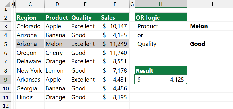

Explanation: We set the lookup value to “1” since we find the TRUE value in a range. The lookup array is a boolean OR expression. The return value can be TRUE or FALSE based on the boolean logic. The lookup array is a named range, “Sales“, that refers to F3:F11.

How to use boolean expressions inside an XLOOKUP formula? The “*” symbol performs a multiplication using the “AND” logical operator. The “+” symbol refers to the “OR” operator.

The formula takes the Product array in column D and finds the first value where the Product equals “Melon”. Since we use an OR logic, the first match is the result. In the example, the third row met the condition.

XLOOKUP across multiple Worksheets

You can use the function across multiple Worksheets easily. We want to summarize and collect data across three Worksheets in the example. All worksheets use the same structure. The first column contains the product name, and the second contains the cost.

First, create three named ranges: Products1, Products2, and Products3, for the sales range, use Cost1, Cost2, and Cost3.

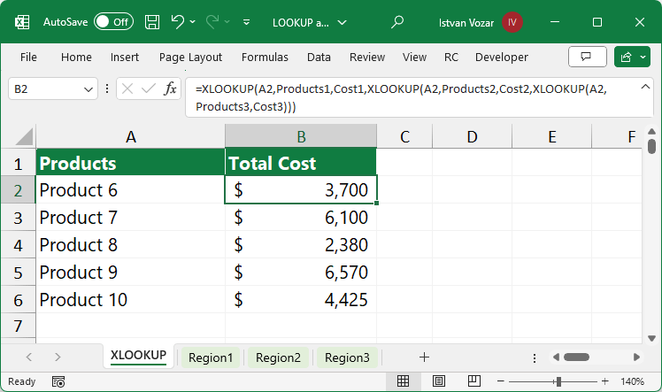
Formula:

=XLOOKUP(A2,Products1,Cost1,XLOOKUP(A2,Products2,Cost2,XLOOKUP(A2,Products3,Cost3)))

Explanation: The nested formula takes the given range across multiple Worksheets and returns the result for all products.

Find the 2nd or nth match using XLOOKUP

This example will demonstrate how to find the 2nd match in an array. Even if you are an advanced user, getting the 2nd match using a custom formula is difficult. To find the second occurrence using the Excel SORTBY function, use the formula below:

=XLOOKUP(G2&G3,Region&
   SORTBY(SEQUENCE(ROWS(Region),1,2)-MATCH(SORT(Region),SORT(Region),0),
   SORTBY(SEQUENCE(ROWS(Region),1,2),Region,1),1),sales)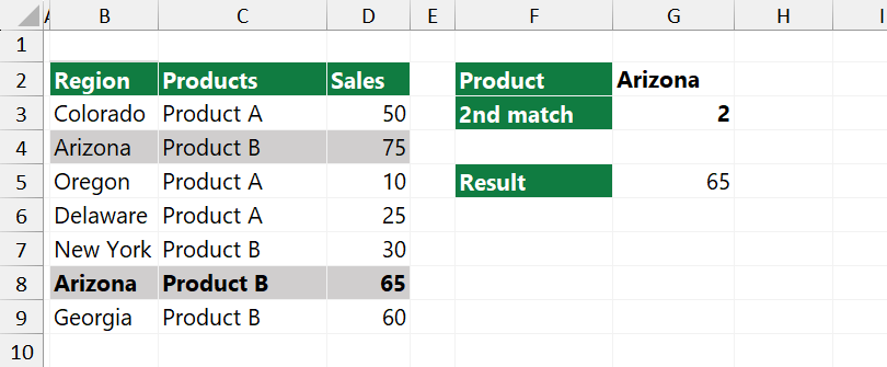

Explanation: First, we need to create the lookup value manually. Concatenate the Region (Arizona) and the nth value using an ampersand (&). For the lookup array, we define a temp array. The reason for using an additional array is that it stores the nth occurrence. To construct the lookup array, use the result of the SORTBY formula. The last step is to add the return array argument, which is the range of “Sales”.

Get the first text value

We aim to extract the first text value in a range in the example. Since XLOOKUP has a wildcard character match mode, we can easily find the first text value in a range containing numeric and text values.

Configure the arguments:

• lookup value = “*”
• lookup array = C3:C10
• return array = C3:C10
• match mode = 2

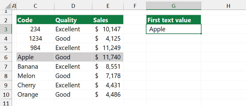
Formula:

=XLOOKUP("*",C3:C10,C3:C10,,2)

Find the first or last positive value in a list

Sometimes, you need to find the first positive value in a list. To perform a text-based search, combine the XLOOKUP and SIGN functions. In Excel, the SIGN function returns the sign of a number. Use “1” as a lookup value!

The goal is to find the first positive numeric value in the column “Profit“. The “Profit” range refers to E3:E10.

Formula:

=XLOOKUP(1,SIGN(Profit), Profit)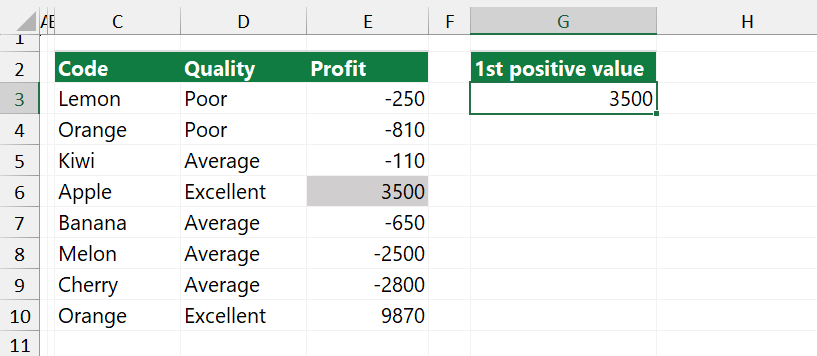

To find the last positive value in a list, set the search mode argument to -1.

=XLOOKUP(1,SIGN(Profit), Profit,,,-1)

Note: To get negative values or zeros in a list, use the -1 or 0 arguments; the logic is the same.

XLOOKUP return blank if blank

Your data range may contain blank cells in the lookup array. This section will show you how to deal with blank cells. It is good to know that the function returns “0” if no value is available in the lookup array. In the example, we use the following arguments:

• Lookup value = “Oregon”
• Lookup array: “Region” (C3:C11)
• Return array: “Sales” (F3:F11)

Enter the formula:

=XLOOKUP("Oregon", Region, Sales)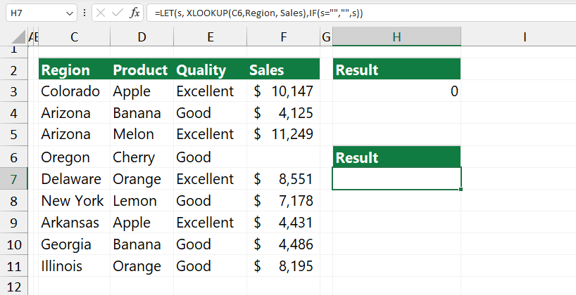

The result is 0 since the corresponding cell is blank. What if you want to return an empty cell if the cell is blank? We combine the XLOOKUP function with the LET and IF functions to show a blank cell if the lookup array contains blank cells.

With the help of the LET function, we can declare a new variable. The formula in cell H7 looks like this:

=LET(s, XLOOKUP(C6,Region, Sales),IF(s="","",s))

In a nutshell: Create a variable, in the example, “s”. Assign the result value to s. If the result is equal to an empty string, the formula returns an empty string (“”). Else, we display the original value.

XLOOKUP Case-sensitive

The example will show you how to use XLOOKUP for case-sensitive matches. By default, the function is not case-sensitive. What does it mean in practice? If your lookup value is “Apple” and the first match is “APPLE”, the formula will ignore the case and returns the first match.

To perform a case-sensitive lookup, we use the EXACT function and create a helper array. In the example, the lookup value is “DELAWARE”.

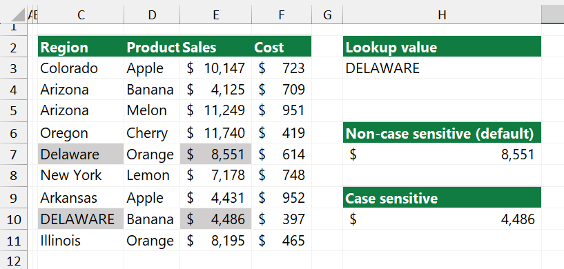
To get the sales for “DELAWARE”, use the formula below:

=XLOOKUP(1, --EXACT(Region,H3),Sales)

Evaluate the formula from the inside out! The EXACT function returns an array that contains TRUE and FALSE values. The double negative method converts TRUE or FALSE values into 1s and 0s.

The formula that uses the converted array looks like this:

=XLOOKUP(1, {0; 0; 0; 0; 0; 0; 0; 1; 0}, Sales)

The result is found in row 8, which is 4486.

XLOOKUP vs. VLOOKUP – Head-to-head comparison

The following list compares the XLOOKUP and VLOOKUP functions, making it easy to decide which is better for you.

1. Multi-direction lookup. XLOOKUP can search horizontally and vertically, replacing the VLOOKUP, HLOOKUP, LOOKUP, and INDEX + MATCH.
2. Support left search. VLOOKUP only searches left to right; XLOOKUP is more flexible. However, you can use a workaround with the CHOOSE function to replace columns on the fly.
3. Return an exact match by default. VLOOKUP provides an approximate match by default. In 99% of queries, we want to find the exact match. So, to make your work easier, use the latest Excel functions.
4. Powerful error handling: You can customize an error message instead of using extra functions, like IFNA. Use the “if not found” argument to improve the readability.
5. Partial match with wildcards. The function provides a useful wildcard match argument for the “match text contain”-type queries.
6. Last-to-first search. Use the search mode argument to reverse the search. Set the argument to 1, and XLOOKUP returns the last match.
7. Return entire columns or rows: Instead of using VLOOKUP or the INDEX + MATCH formula, XLOOKUP can return an entire row or column.
8. Multiple criteria support: Use multiple criteria to construct a lookup value: concatenate multiple lookup values to join them into a single value.
9. High Performance (Binary search): When working with large data sets, it is worth using a binary search since it is much faster than other methods.

You can learn more about the function by reading our definitive guide.

Why is XLOOKUP not working properly?

Sometimes, your function is not working in Excel. This section will explain how to avoid the most common errors. Furthermore, we show you the workarounds regarding errors.

Here are the top 10 reasons why XLOOKUP is not working properly:

1. Not supported
2. Different array sizes
3. Invalid arguments
4. No exact match: Missing error handling argument
5. No approximate match
6. Different data types
7. Non-printable characters in lookup arrays
8. Binary search with unsorted records
9. Typo, missing named ranges, commas
10. The dynamic array contains data (#SPILL error)

#1: Function is not supported

Check your Excel version if you are not a Microsoft 365 or Excel 2021 subscriber. Open Excel > Click File > Account. Check the product information dialog box. Use an Excel add-in that provides backward compatibility if your Excel version is unsupported. The add-in works fine with all Excel versions.

#2: Different array sizes

Row or column size differences cause a #VALUE error. Make sure that the lookup value and lookup array sizes are the same. We recommend you use the TRANSPOSE function to change a 10×1 array to 1×10. Click the formula bar and manually check the equal range sizes; Excel highlights the selected array.

#3: Invalid arguments

The function uses the optional match mode and search mode arguments. The match mode handles the following values only: 0, -1, 1, and 2. The search mode arguments use 1, -1, 2, and -2 to control the search. Make sure that all arguments are valid to avoid #VALUE errors.

#4: No Exact match: Missing error handling argument

As we stated above, the function returns an #N/A error if no exact match is found. We recommend writing better formulas using the 4th “if not found” argument. In this case, you can replace the #N/A error with “not found” or “no matching record found”.

#5: No approximate match is found

For example, set the match mode argument to -1 to get the next smaller item (approximate match. Excel evaluates the formula. If no exact match is found, it returns the next smaller match from the lookup array. What if all values are greater than the lookup value? Since no exact or approximate matches are found, it returns an #N/A error.

#6: Different Data Types

It is good to know that you must use the same data types regarding lookup value and array. Let us suppose that the lookup value is numeric, but you try to use it in an array that contains text values. Since we have different data types, the formula returns with an #N/A error.

In this case, we recommend you double-check the small green triangle. The marker should appear on the top-left corner of the cell. Use the “Convert to Number” command to fix the formula.

#7: Non-printable characters in lookup arrays

Non-printable characters may cause #N/A errors too. It is hard to identify that the cell contains spaces or unwanted characters. The best solution is to clean your data first. You can use various text-cleaning functions, like TRIM. Do not forget: “value “ is not equal to “value”. The first string contains extra spaces.

#8: Binary search with unsorted records

The binary search mode is fast when working with large data sets. Ensure the data is sorted before using the “2” or “-2” values as a 6th argument. The best practice is to sort the data using the SORT and SORTBY functions.

#9: Typo, missing named ranges, commas

Last but not least, we have to talk about typos. Please carefully use names in the following cases:

• Incorrect usage of function names, like “X-LOOKUP“
• Named ranges (Sales instead of Sales_)
• Semicolon instead of a comma or vice versa

In all the above-mentioned cases, you will get the #NAME error. You can check the integrity of named ranges using the Formulas tab > Name Manager. You can separate the arguments using a comma or a semicolon. The separator character depends on your Excel version. Most Excel versions use a comma by default. The international versions of Excel use a semicolon.

#10: The output array contains data (#SPILL error)

In the era of dynamic array functions, the formula may return with a #SPILL error. The reason for the issue is simple: The result array can not overwrite the cells if they contain data. To identify and fix the error, move the cursor over the output range and click the yellow triangle.

Excel shows the following error: “A cell we need to spill data into is not blank”. Ensure that the output range is blank and contains no data.

Wrapping things up

Thanks for being with us today. It is the right time to start using the function. Check the video tutorial below. The video demonstrates the most used examples. Stay tuned.