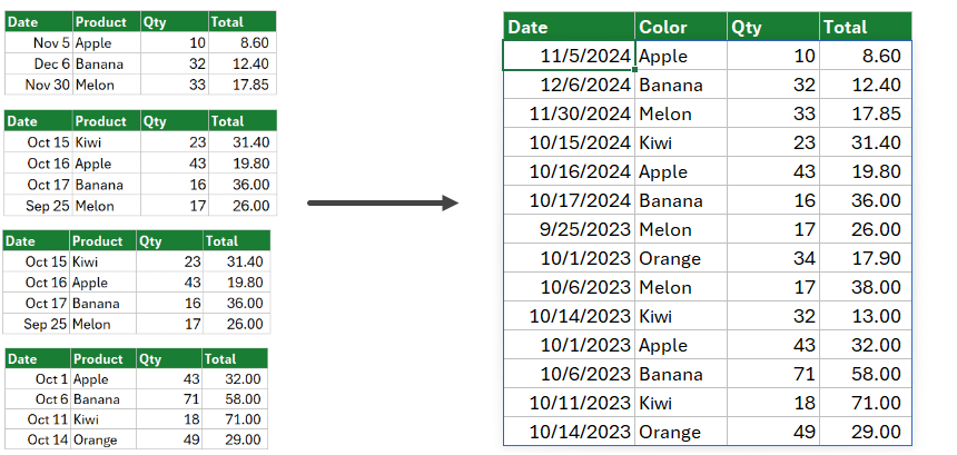
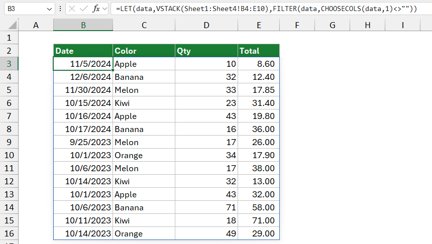
To combine data in multiple worksheets, you can use a formula based on the VSTACK, LET, FILTER, and CHOOSECOLS functions.
How to combine data in multiple Worksheets?
- Open Excel.
- Type =LET(data,VSTACK(Sheet1:Sheet4!B4:E10),FILTER(data,CHOOSECOLS(data,1)<>””))
- Press Enter.
- This formula stacks the specified range from Sheet 1 through Sheet 4.
Example
The formula example demonstrates using the VSTACK and FILTER functions to combine data from multiple sheets, remove empty rows, and consolidate the information into a single table.
- Goal: To extract data from Sheet1 to Sheet4, ignoring any empty rows, and merge it into a single table.
- Input Data: Each sheet (Sheet1 to Sheet4) contains a table with columns Date, Product, Qty, and Total, each with some rows.
- Output Data: A consolidated table with non-blank rows only, providing a unified view of all products, quantities, and totals.
Formula:
=LET(data,VSTACK(Sheet1:Sheet4!B4:E10),FILTER(data,CHOOSECOLS(data,1)<>””))

Explanation
Take a closer look at the formula and evaluate it from the inside out:
Formula:
=LET(data,VSTACK(Sheet1:Sheet4!B4:E10),FILTER(data,CHOOSECOLS(data,1)<>””))
- LET(data, …): The LET function creates variable data to store the result of a calculation, making it easier to reference this result throughout the formula.
- VSTACK(Sheet1:Sheet4!B4:E10): The VSTACK function stacks data from the range B4:E10 across multiple sheets (Sheet1, Sheet2, Sheet3, and Sheet4) into one continuous array. Essentially, this pulls all data from these sheets into a single, unified dataset.
- FILTER(data, CHOOSECOLS(data,1)<>””): After combining the data, FILTER extracts only the rows where the first column is not blank.
- CHOOSECOLS(data,1): This picks the first column of the data array.
- <>””: The <>”” condition checks for non-blank entries.
The formula consolidates data from the specified range across four sheets, filtering out rows with blank cells in the first column. This is useful for merging data from multiple sheets into a single list, only retaining rows with entries in the first column.
Combine data without using the LET function
Note: By eliminating LET, this version directly references VSTACK twice. While it’s still efficient, the readability might be slightly reduced compared to the LET version, especially if the formula grows more complex.
=FILTER(VSTACK(Sheet1:Sheet4!B4:E16), CHOOSECOLS(VSTACK(Sheet1:Sheet4!B4:E16), 1) <> “”)
You can download the practice file with the solution.
