To combine or consolidate ranges in Excel, you can use a formula based on the VSTACK function or the HSTACK function.
How to combine ranges in Excel
Here are the steps to combine ranges vertically or horizontally:
- Open Excel
- Type =VSTACK(range1, range2) to combine ranges vertically.
- Type =HSTACK(range1, range2) to combine ranges horizontally.
- Press Enter.
- The formula will return all columns combined into one range, aligned vertically or horizontally.
Generic Formula
=VSTACK(range1, range2)
The =VSTACK(range1, range2) formula is part of the new Excel dynamic array functions, designed to simplify combining data arrays.
Consolidate ranges vertically
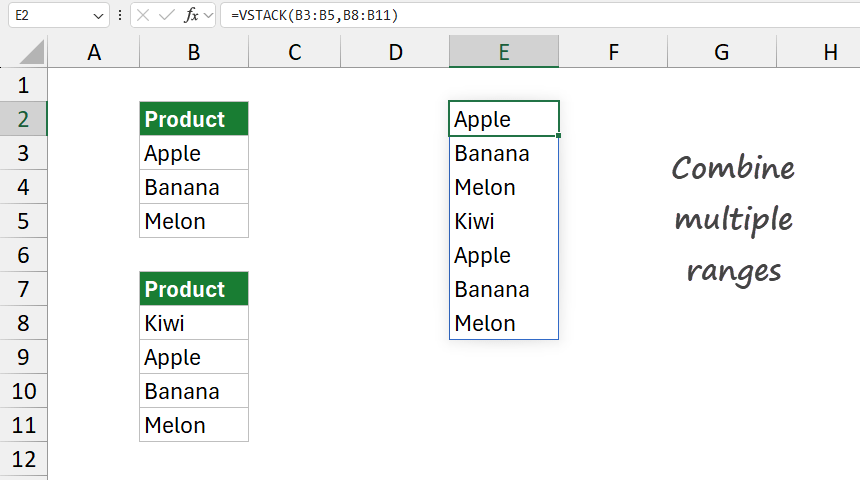
In the example, try to combine the B3:B5 and B8:B11 ranges.
VSTACK is a dynamic array function in Excel that takes multiple ranges and stacks them on top of each other in a single column. In the example provided, VSTACK combines the products from two different ranges into one continuous list in column E.

This method works fine in Microsoft 365 or Excel 2019, where dynamic array functions are supported. For older versions, you would need to copy and paste each range to combine them manually.
Combine ranges horizontally
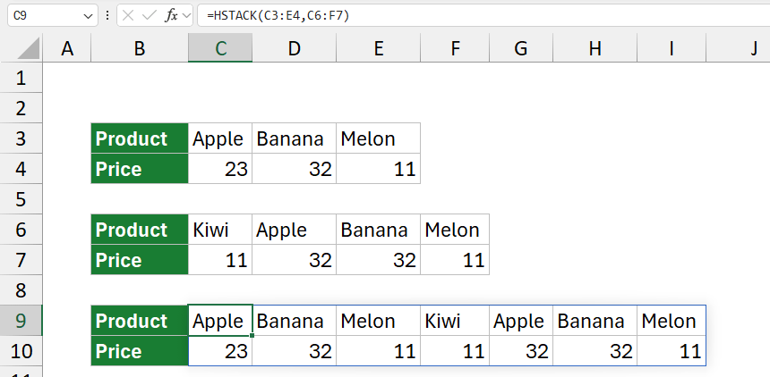
If you have horizontally arranged data, you can use the HSTACK function to create a single array.
Formula:
=HSTACK(C3:E4,C6:F7)

Note: VSTACK and HSTACK are dynamic array functions; the formula appends the second range to the first range, and the result spills into C9:I10.
Combine multiple column ranges
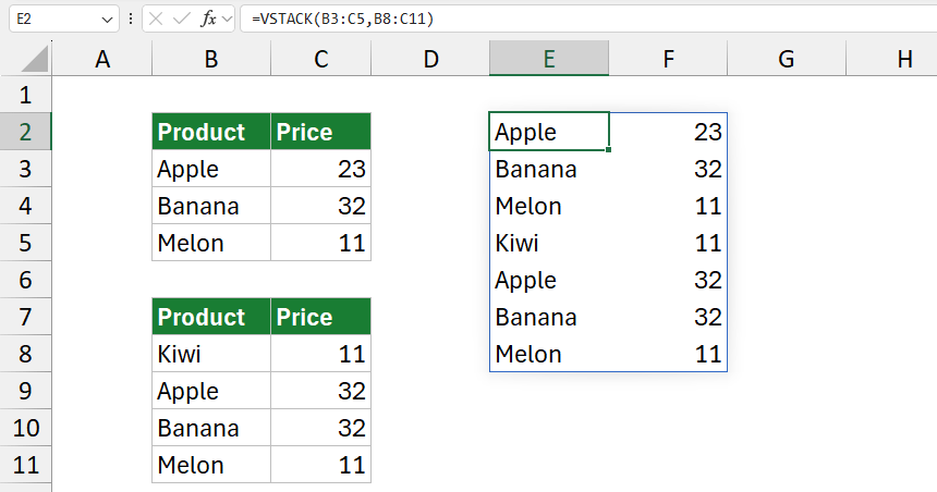
Sometimes, we need to work with custom data structures. In the example, the goal is to merge ranges with multiple columns. The formula =VSTACK(B3:C5, B8:C11) combines multiple ranges vertically, stacking them one below the other into a single array.

In this case, the formula appends the second range (B8:C11) to the first range (B3:C5), and the result spills into E2:F8.
Download the practice file and play with the formulas.
Related formulas
- Combine data in multiple Worksheets
- Combine multiple Workbooks
- Get unique values from multiple ranges