To count rows that meet two or more specified criteria, you can use a formula based on the versatile COUNTIFS function.
How to count rows based on two criteria?
Here are the steps to count rows based on multiple criteria in Excel:
- Open Excel.
- Type: =COUNTIFS(B3:B11,”Orange”,C3:C11,”>55″)
- Press Enter.
- The formula returns the count of rows that meet both specified criteria.
Example
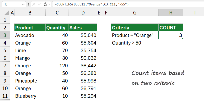
In the example, we have sales data in range B3:D11.
Formula:
=COUNTIFS(B3:B11,”Orange”,C3:C11,”>55″)
In this example, we want to count rows where the Product is “Orange” in column B and the Quantity is greater than 55 in column C. The COUNTIFS function allows us to specify multiple criteria in pairs — each pair consists of a range and a condition that applies to that range.

The result is 3, since there are three rows with a product of “Orange” and quantity greater than 55.
Example rows that meet the criteria:
- Row 4: Orange with quantity 60
- Row 7: Orange with quantity 120
- Row 9: Orange with quantity 60
Explanation
Take a closer look at the formula.
COUNTIFS Function:
The COUNTIFS function counts cells based on multiple criteria. Each criterion is applied to a specific range, and only rows meeting all criteria are counted. Here, COUNTIFS will only count rows where both conditions are true.
First criteria pair, (B3:B11, “Orange”):
- Range: B3:B11 (Product column).
- Condition: “Orange”. This part of the formula checks each cell in B3:B11 to see if it contains the word “Orange”. If the cell contains “Orange”, it is included in the count for this criteria.
Second criteria pair, (C3:C11, “>55”):
- Range: C3:C11 (Quantity column).
- Condition: “>55”. This part checks each cell in the C3:C11 range to see if it is greater than 55. Only rows with a quantity above 55 meet this condition.
The formula returns 3 because there are three rows in the data where the product is “Orange” and the quantity is greater than 55.
Combined criteria:
The COUNTIFS function will only count rows where both conditions are met simultaneously. So, it will only count rows where the product in column B is “Orange”, and the quantity in column C is greater than 55.
Using Dynamic Ranges with Named Ranges
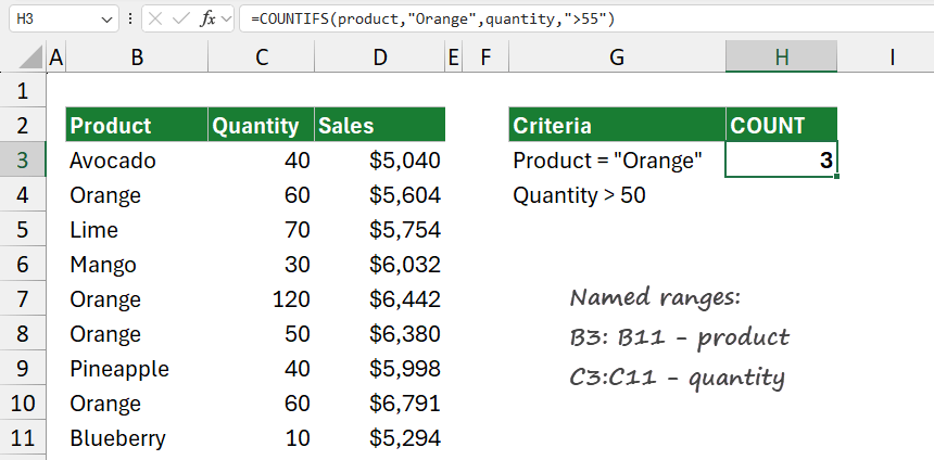
You can define named ranges for “Product” and “Quantity” to make the formula more readable.
Formula:
=COUNTIFS(Product, “Orange”, Quantity, “>55”)

Adding more criteria (Optional):
You can add more criteria by adding range-criteria pairs to the COUNTIFS function.
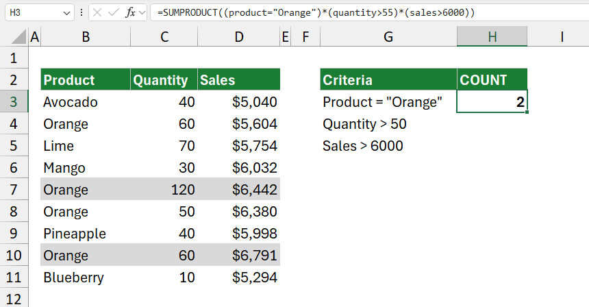
For example, =COUNTIFS(B3:B11, “Orange”, C3:C11, “>55”, D3:D11, “>6000”) will count only rows where the product = “Orange”, Quantity is greater than 55 and “Sales” (in column D) are greater than 6000.
Workaround with SUMPRODUCT
For users familiar with the SUMPRODUCT function, you can achieve the same result using the following formula:
=COUNTIFS(product, “Orange”, quantity, “>55”, sales, “>6000”)

This formula counts rows that meet all three conditions.
You can download the practice file here.