To count matches between two columns in Excel based on the corresponding rows, you can use the SUMPRODUCT function.
How to compare two columns and count matches?
- Open Excel.
- Type the formula =SUMPRODUCT(–(range1 = range2)).
- Press Enter.
- This formula will also count the matches between the two columns row by row.
Example
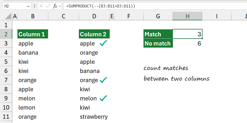
In the example, we want to compare two columns and write a formula to count matches and differences.
Formula:
=SUMPRODUCT(–(B3:B11=D3:D11))

The formula returns with 3, so we have three matching records.
Explanation
Evaluate the formula!
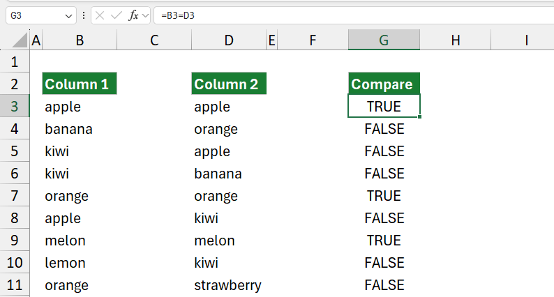
=B3=D3:
This part checks if each cell in B3:B11 matches the corresponding cell in D3:D11. The “=” operator creates a comparison, resulting in an array of TRUE or FALSE values. For example: If B3 and D3 contain “apple,” the comparison B3=D3 will be TRUE. If B4 contains “banana” and D4 contains “orange,” the comparison B4=D4 will be FALSE.
The result array from this part will look like {TRUE, FALSE, FALSE, FALSE, TRUE, TRUE, FALSE, FALSE, FALSE}.

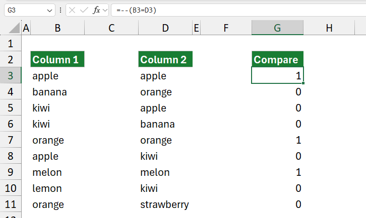
–(B3=D3):
The double negative method converts TRUE and FALSE values into 1 and 0. TRUE becomes 1, and FALSE becomes 0, so the array from the previous step becomes {1, 0, 0, 0, 1, 1, 0, 0, 0}. This transformation allows us to count the matches as numbers.

=SUMPRODUCT(–(B3=D3)):
SUMPRODUCT takes the array {1, 0, 0, 0, 1, 1, 0, 0, 0} and sums up the values. Since each 1 represents a match, the sum will be the total count of matching items in the two columns. In this example, the result is 3, meaning there are three matches between B3:B11 and D3:D11.
If you want to compare two columns and find the non-matching records, use the following formula:
=SUMPRODUCT(–(B3:B11<>D3:D11))
You can also use the SUM function to count matches in Microsoft 365 (we have native dynamic array support).
=SUM(–B3:B11=D3:D11)) or =SUM(–B3:B11<>D3:D11))