How to extract word from string in Excel: first, last, or nth

This tutorial will show you straightforward ways to extract a word or words in Excel without using complex formulas.

When working in Excel, the data often comes in a raw format and needs cleaning before analysis. The goal is to extract the specified word or words and transform strings into a more straightforward, standardized format. For example, a cell might contain full names but only need the first name.

Sometimes, you need to extract the first or the last word only. But some advanced task requires complex formulas. For example, you want to find the nth word in a text or get the first “n” words. We will show you powerful functions to perform these time-consuming tasks.

This comprehensive guide will introduce all methods for extracting a word from a cell containing a string. We prepared a practice file containing all string manipulation functions for time-saving purposes. You can download the Worksheet and use it freely.

Table of contents:

1. How to extract word from a string in Excel
2. Extract the first word from a string
3. Get the last word from a string
4. Using the GETLASTWORD function to strip the last word
5. Extract the first N words from a text
6. Return the nth word
7. Extract the nth word using built-in functions
8. Extracting words with custom delimiter
9. Extract a word containing specific text
10. Extract and split words into multiple cells

How to extract word from a string in Excel

There are various ways to extract a word from a text. You can use built-in Excel functions to construct advanced formulas. However, the best way is to write a custom function for the specific task. The main advantage of this method is that you can store the code inside an add-in. As a final step, you can share your work easily.

Extract the first word from a string

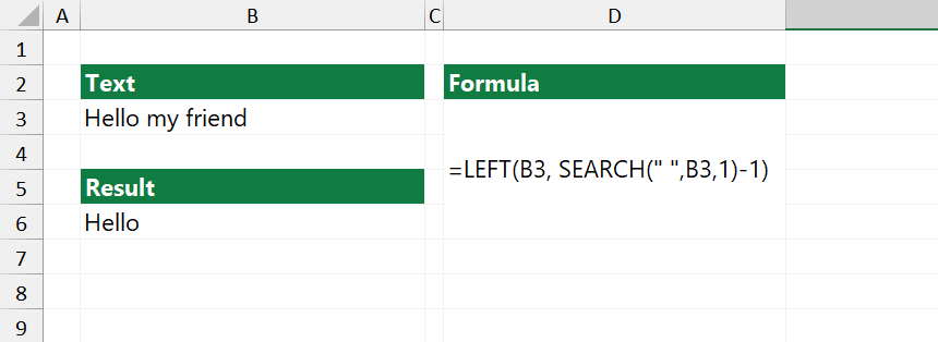
If you want to extract the first word from a text string in an Excel cell, you can combine the LEFT and SEARCH functions. In the example, cell B3 contains the text “Hello, my friend”, and you want to extract the first word using regular Excel functions.

Steps to extract the first word from a string:

1. Select cell B6.
2. Type the formula: =LEFT(B3, SEARCH(” “,B3,1)-1)
3. Press Enter.
4. Excel will return the first word.

Explanation:

• FIND or SEARCH functions are used to locate the first space (“”) in the text, which usually indicates the end of the first word.
• The LEFT function is then used to extract all characters before this position.
• We subtract 1 from the position to exclude the space from the extraction.

Note: If the cell may not contain any spaces, the formula will return an error because FIND and SEARCH will not locate a space. Use an error-handling function:

=IFERROR(LEFT(B3, SEARCH(” “,B3,1)-1), B3)

If you prefer VBA, you can use this code:

Function GETFIRSTWORD(text As String) As String
Dim arr() As String
arr = Split(text, " ")
GETFIRSTWORD = arr(0)
End Function

Explanation: The function splits the text string into an array using space as a delimiter and creates an array from the result. If the cell is empty or doesn’t contain any space, it will return the whole content of the cell. It’s a small but powerful string manipulation function.

Get the last word from a string

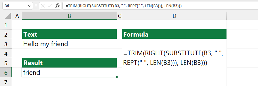
You can use built-in Excel functions to extract the last word from a string. You want to get the last word from cell B3 in the example. Next, return the first element in the array, which is the first word in your text.

Formula:

=TRIM(RIGHT(SUBSTITUTE(B3, ” “, REPT(” “, LEN(B3))), LEN(B3)))

Explanation:

1. =SUBSTITUTE(text, old_text, new_text, [instance_num]) replaces occurrences of a specified text within a cell with a new text.
2. =REPT(text, number_times) returns a text string that is the first argument repeated as many times as specified in the second argument.
3. In the example, SUBSTITUTE replaces each space (“”) in your cell B3 with several spaces equal to the length of the text in B3.
4. =LEN(B3) gets the length of text in B3, and REPT repeats a space that many times. This step separates each word in the original cell with several spaces. After the SUBSTITUTE function works, each word in the original string is separated by spaces.
5. =RIGHT(text, [num_chars]) extracts a certain number of characters from the right side of a text string.
6. =RIGHT(SUBSTITUTE(B3,” “, REPT(““, LEN(B3))), LEN(B3)) is taking the string of words separated by multiple spaces and extracting characters from the right, based on the length of the original text (which is the number of characters specified). Because of how the spaces were inserted, this will include the last word plus several spaces before it but no complete words before that.

After the RIGHT function gets the last word and several spaces, there are still all those extra spaces to deal with. This is where TRIM(text) comes in. TRIM removes all spaces from a text string except for single spaces between words.

Using the GETLASTWORD function to strip the last word

The GETLASTWORD function is an effective UDF; use it to save time. Let us see how easy it is to produce the result using the previous example:

=GETLASTWORD(“Hello my friend”)

If you want to implement the function, copy and paste the code below:

Function GETLASTWORD(string1 As String)
Dim str As String
str = StrReverse(string1)
str = Left(str, InStr(1, str, " ", vbTextCompare))
GETLASTWORD = StrReverse(Trim(str))
End Function

Extract the first N words from a text

As we stated above, you can save time using user-defined functions. For example, the GETNWORDS function offers powerful customization, not just for advanced users. It helps you to extract the first N words from the beginning of a text string.

Syntax: GETNWORDS(text, n)

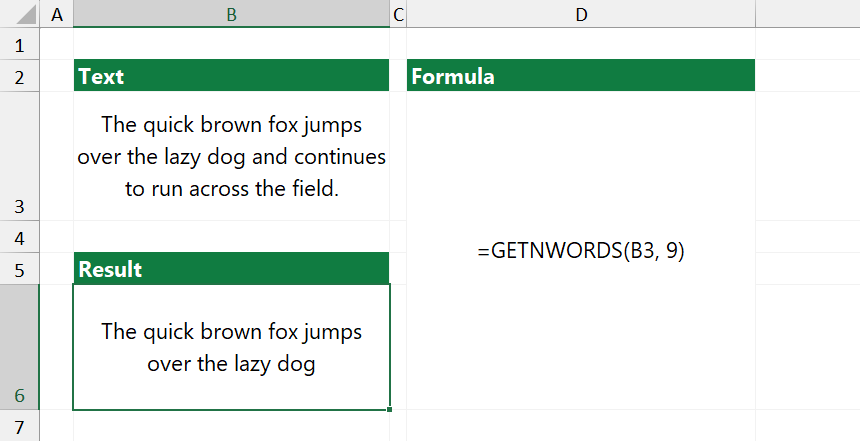
In cell B2, you have a string of text: “The quick brown fox jumps over the lazy dog and continues to run across the field.”

Steps to extract the first N words from a text:

1. Click the cell B6.
2. Type the formula: =GETNWORDS(B3, 9)
3. Press Enter.
4. The formula will return the first 9 words.

First, the formula takes the contents of B3 (our sentence about the fox and the dog) and the number 9. After that, split the text into individual words and take the first nine words from the entire text.

Result: “The quick brown fox jumps over the lazy dog”, this is the first nine words of the original string.

How the GETNWORDS function works?

1. GETNWORDS takes two arguments: ‘text’ (the cell that contains text) and ‘num_of_words’ (an integer representing the number of words you want to extract from the text). The function returns a string, the first num_of_words words of the text.
2. Error handling: The function returns an empty string if the number of word arguments is less than or equal to 0.
3. Split the text into words: The UDF uses the split function to divide the text into individual words, splitting them at each space character (“”). The output is an array containing words.
4. A loop runs until the ‘I’ variable is less than ‘num_of_words’.
5. The UBound function returns the upper index of the words() array. Each iteration adds the next word to the result, separated by a space.
6. The result is a string, the input text’s first ‘num_of_words words’.

Return the Nth word

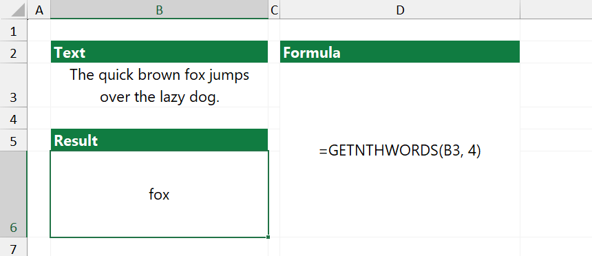
In the example, cell B3 contains the string, “The quick brown fox jumps over the lazy dog.” To extract the nth word from a text, you can use the GETNTHWORDS function.

Steps to return the nth word in Excel:

1. Select cell B6.
2. Type the formula: =GETNTHWORDS(B3, 4).
3. Press Enter.
4. The formula returns the fourth word.

For example, =GETNTHWORDS(B3, 4) would return the fourth word in the text in cell B3.

Explanation:

The GETNTHWORDS function checks every letter in the cell. It starts collecting letters together to create words. If a space character is found, examine if this is the word number you wanted (based on the “n” value). In case of yes, it returns the given text. Otherwise, it checks the next word until it finds the right word and ensures no extra spaces exist.

The function scans through the input text, carefully stepping from one word to the next until it finds and extracts the specific word you specified.

Extract the nth word using built-in functions

You can extract the nth word using a combination of built-in functions.

In the example:

=TRIM(MID(SUBSTITUTE($B$3,””,REPT(” “,LEN($B$3))),(n-1)LEN($B$3)+1,LEN($B$3)))

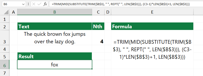
So, if you want to extract the 4th word, use the formula below:

=TRIM(MID(SUBSTITUTE(TRIM($B$3), ” “, REPT(” “, LEN($B$3))), (C3-1)*LEN($B$3)+1, LEN($B$3)))

Evaluate the formula from the inside out:

1. SUBSTITUTE($B$3,”” ,REPT(““, LEN($B$3))) replaces every instance of the asterisk”” in the text in B3 with a number of spaces equal to the length of the text in B3.
2. REPT(““,LEN($B$3)) generates a text string consisting of spaces. The number of spaces is the same as the number of characters in B3.
3. SUBSTITUTE replaces each “” with that string of spaces, effectively spreading out the segments of the original text so they are each as long as the original text and are separated by spaces. MID(text, start_num, num_chars) extracts a substring from the middle of a text string, starting at start_num and taking num_chars characters. (C3-1)LEN($B$3)+1 calculate the start_num.
4. LEN($B$3) is the num_chars, specifying the substring length you want to extract.
5. TRIM() removes any leading, trailing, or multiple spaces between words, leaving only single spaces between words and no spaces at the start or end of the text. The goal is to clean up the result from the MID function.

Extracting words separated by a custom delimiter

In most cases, you use space as a separator between words. However, Excel data often comes from another source and contains custom separators like semicolons, slashes, or non-printable characters. What if we have a text with delimiters like the following characters: “/”, “*”, “-“, “&”.

The GETWORDS function is designed to split a text string into ‘words’ based on a specified delimiter and then return the word at the position you indicated.

Steps to extract words with custom delimiter:

1. Select cell B3
2. Type the formula: GETWORDS(B3, 2, “*”)
3. Press Enter
4. The formula extracts the 2nd word after the custom delimiter.

Syntax:

=GETWORDS(cell, n, delimiter)

Arguments:

• “cell” refers to the single cell containing text.
• “n” indicates the position of the word you want to extract from the text.
• “delimiter” represents the character or string that separates words in the cell text.

Example:

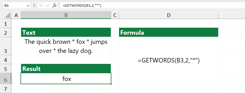
=GETWORDS(B3,2,”*”)

Explanation:

• B3 is the cell reference, so the text string that the function analyzes is the content of B3.
• 2 is the word number you want to retrieve. You’re asking the function to get the second ‘word’ from the split text.
• “*” is your delimiter. The function splits the text into ‘words’ whenever it finds the asterisk () character.

It splits the text from B3 into words wherever it sees your delimiter, the asterisk (*). So, the segments look like:

1. “The quick brown “
2. ” fox “
3. ” jumps over “
4. ” the lazy dog.”

It then looks to return the second segment from this split, as you’ve specified 2 for the word number. The first part is “The quick brown “, and the second part is ” fox “.

How to extract words containing specific text

For example, to identify and extract email addresses from a text, you can use the WORDCONTAINS function. If you have the text “Contact [email protected] / Date 12/12/2022” in cell B3. This function is useful for quickly parsing text in a cell to find specific substrings or “words” that contain a given character, like “@” for email addresses.

Formula:

=WORDCONTAINS(B3, “@”)

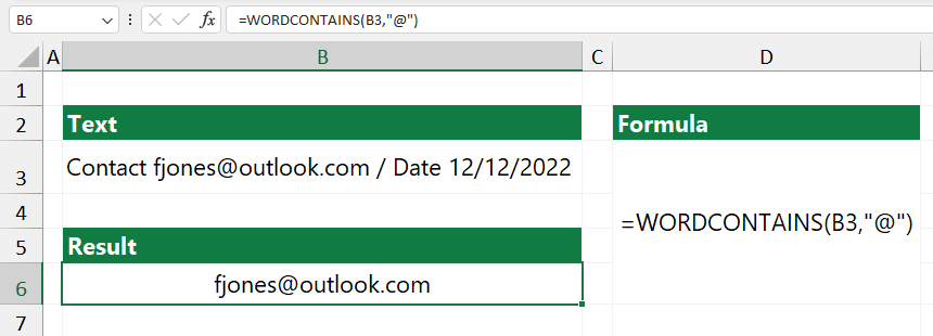
The function will search for any word in cell B3 that contains the “@” character. In this case, it will find and return the email address.

Extract and split words into multiple cells

In Excel 2019 and Microsoft 365, you can use dynamic array functions.

Steps to split words into multiple cells:

1. Select cell B5
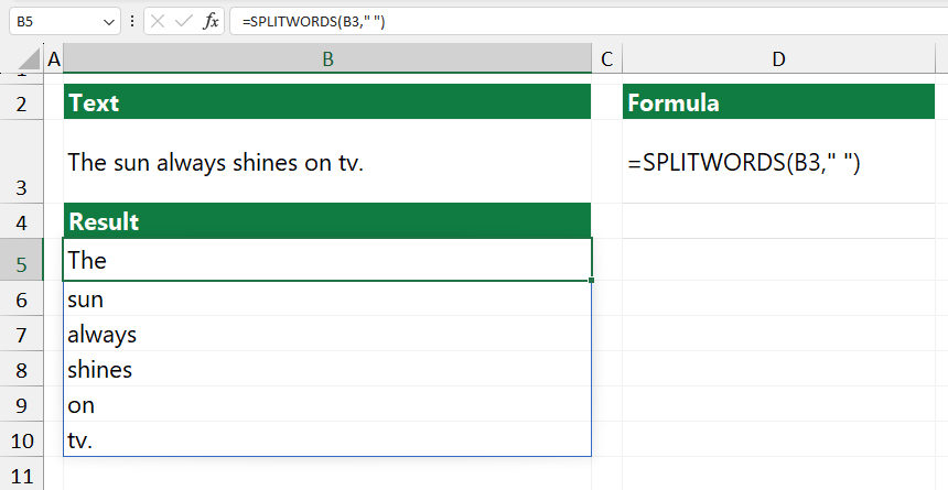
2. Type the formula: =SPLITWORDS(B2,” “).
3. Press Enter
4. SPLITWORDS will spill the results to the cells below B5, splitting the text based on spaces and creating a vertical list.

Related Formulas

• Separate names (first, last and middle)
• Excel SUBSTRING function examples
• How to extract a number from a string