To filter data with a case-sensitive method in Excel, you can use a formula based on the FILTER and the EXACT function.
How to use a case-sensitive filter?
Here are the steps to use the FILTER function in Excel for a case-sensitive filter:
- Open Excel.
- Type =FILTER(data, EXACT(data, “criteria”)).
- Press Enter.
- The formula will return a filtered list matching the exact, case-sensitive text in the specified range.
Example
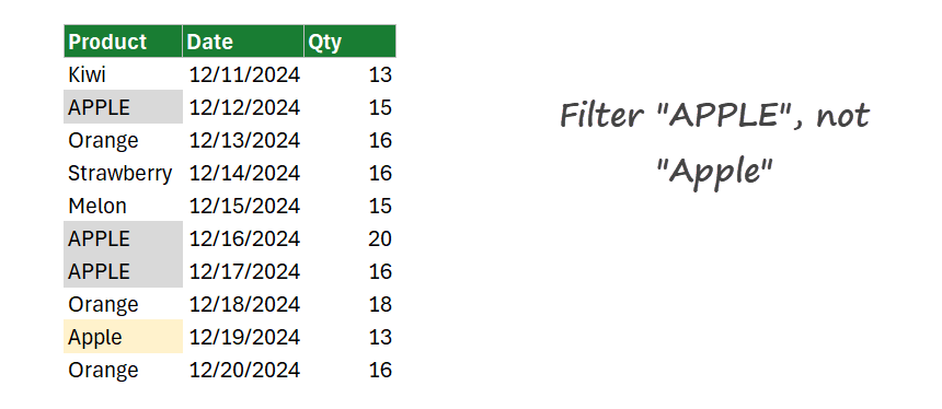
In the example, the goal is to filter data based on product. The product name should be case-sensitive.

Formula:
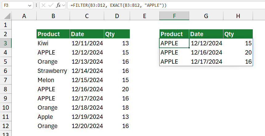
=FILTER(B3:D12, EXACT(B3:B12, “APPLE”))
Result:

Explanation
This formula =FILTER(B3:D12, EXACT(B3:B12, “APPLE”)) uses the FILTER function to extract data based on a case-sensitive condition. The data range, B3:D12, includes all rows without headers. The include argument relies on the EXACT function, which performs a case-sensitive comparison between two text strings. When two strings match exactly, EXACT returns TRUE; if not, it returns FALSE.
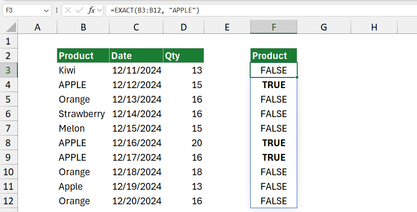
EXACT compares each value in the range with the string “APPLE”, resulting in an array of 10 TRUE or FALSE values. Positions with TRUE align with rows where the product name is “APPLE”.

This array is passed to FILTER as the include argument, directing FILTER to display only rows from B3:D12 where the product name is “APPLE” exactly. Rows labeled “Apple” are excluded, ensuring case sensitivity in the results.
Partial match case
The EXACT function only returns exact, case-sensitive matches. The EXACT function alone will not work when performing a case-sensitive partial match with FILTER. However, you can use a workaround with SEARCH and FILTER to achieve a case-insensitive partial match and then add logic to make it case-sensitive.
Here’s how to use FILTER for a case-sensitive partial match:
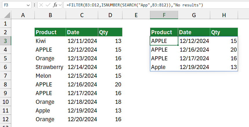
=FILTER(B3:D12,ISNUMBER(SEARCH(“App”,B3:B12)),”No results”)
The formula =FILTER(B3:D12, ISNUMBER(SEARCH(“App”, B3:B12)), “No results”) filters rows from the range B3:D12 that contain the substring “App” (case-insensitive) in column B. If there are no matches, it returns “No results” instead of an error.

In a nutshell:
- SEARCH(“App”, B3): The SEARCH function looks for the substring “App” in each cell within the range B3:B12. It is case-insensitive, so it will match “App,” “app,” or “APPLE,” among other variations.
- ISNUMBER(SEARCH(“App”, B3)): ISNUMBER checks if SEARCH finds a match for “App” in each cell. When “App” is found, SEARCH returns the starting position as a number, and ISNUMBER will return TRUE. If “App” isn’t found, SEARCH returns an error, and ISNUMBER outputs FALSE.
- FILTER(B3, ISNUMBER(SEARCH(“App”, B3)), “No results”): The FILTER function uses the TRUE/FALSE values to include only the rows where ISNUMBER returns TRUE (where “App” was found). If no rows meet this condition, FILTER returns “No results” instead of leaving a blank or showing an error.