To filter data and extract records between two dates, you can use a formula based on the FILTER function with Boolean logic.
How to filter data between two dates?
Here are the steps to filter data between two dates in Excel:
- Open Excel.
- Type =FILTER(data_range, (date_range >= start_date) * (date_range <= end_date)).
- Press Enter.
- The formula filters and displays data between the specified start and end dates.
Example
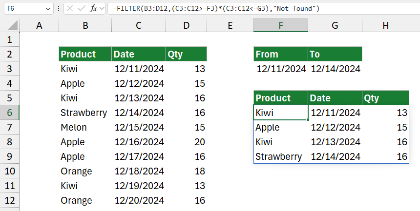
In the example, we have the data in range B3:D12. The goal is to extract records between two dates. The start date is in cell F3, and the end date is in cell G3.
Formula:
=FILTER(B3:D12,(C3:C12>=F3)*(C3:C12<=G3),”Not found”)

The formula =FILTER(B3:D12, (C3:C12 >= F3) * (C3:C12 <= G3), “Not found”) extract rows from the range B3:D12 where the values in the range C3:C12 fall between the criteria specified in F3 and G3.
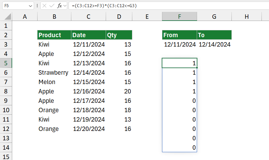
In the formula =(C3:C12 >= F3) * (C3:C12 <= G3) in cell F5, you’re using Boolean logic to check if the dates in C3:C12 fall within a specified range defined by F3 (start date) and G3 (end date).

The first part of the formula (C3:C12 >= F3) checks if each date in the range C3:C12 is greater than or equal to the date in F3. It returns an array of Boolean values: TRUE if the condition is met and FALSE if not. The second part of the formula (C3:C12 <= G3) checks if each date in C3:C12 is less than or equal to the date in G3. It also returns an array of TRUE or FALSE values.
The * sign between these two boolean expressions is an AND logical operator. This multiplication produces an array of 1s and 0s, where 1 represents a row that meets both conditions (falls within the date range), and 0 represents a row that does not.
Explanation
Evaluate the formula:
- Condition: The expression (C3:C12 >= F3) * (C3:C12 <= G3) creates a logical test. It checks if each value in C3:C12 is greater than or equal to the value in F3. Less than or equal to the value in G3. Using the multiplication sign * between these two conditions acts as an AND operator, meaning a row will only pass the filter if both conditions are TRUE for that row.
- FILTER: The FILTER function will include rows from B3:D12 that meet the above condition. If both conditions are TRUE for a row, that row is included in the results.
- If No Match: If no rows meet the criteria, the function returns “Not found,” as specified in the third argument of FILTER.
Why the FILTER function is preferred?
The FILTER function avoids the need for complex array formulas with INDEX and SMALL, which can sometimes misbehave in certain contexts. Since FILTER returns the exact rows that meet your conditions, it’s simpler and more efficient.