This quick guide will show you how to get the nth value in a column using the CHOOSEROWS function in Excel.
How to get the nth value in a column?
Here are the steps to get the nth value in a column:
- Open Excel
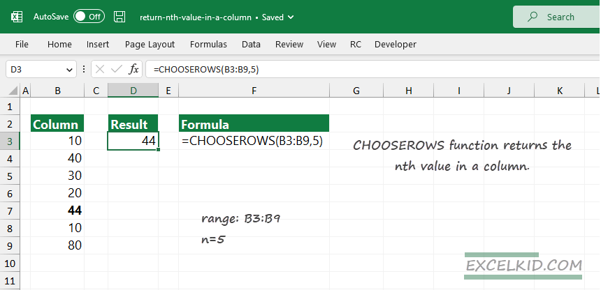
- In cell D3, type =CHOOSEROWS(B3:B9,5)
- Press Enter.
- The formula returns the 5th value in a range.
CHOOSEROWS function
The CHOOSEROWS function returns the specified rows from an array. It requires Excel for Microsoft 365, but there is a workaround with the OFFSET function.
Sometimes, you can use a function for other purposes, not just the primary goal. It is good to know that if you want to extract the nth value in a given column, use the CHOOSEROWS function with the required arguments only.
Syntax:
=CHOOSEROWS(array, row_num1, [row_num2])
Arguments:
CHOOSEROWS uses two required and multiple optional arguments.
- array: the array that contains the nth value (column)
- row_num1: an integer value that represents the nth value
- row_num2: optional argument
Formula Example
Let us see how to write a formula that returns the 5th value in a selected range, B3:B9.
Formula:
=CHOOSEROWS(B3:B9, 5)
Explanation: First, select the range to find the nth value. In the example, B3:B9. Next, set a numeric value (integer) as a second argument. Finally, we want to find the 5th value in the given column. So, add “5” as a row_num1 argument.
Workaround with the OFFSET function
If you are not a Microsoft 365 subscriber, do not worry: you can retrieve the second, third, or fifth value in a column using the built-in OFFSET function, which is compatible with all Excel versions.
Formula:
=OFFSET(B3,4,0,1,1)
Explaining how the OFFSET function works for Excel newbies can be challenging. Here is an easy-to-understand guide.
OFFSET works like a “moving range”. With its help, Excel can return different parts of the Worksheet. The function can return a single value. The reference is the starting point of the selected column, cell B3.
To get the 5th value in the column, we need to shift the range downwards to 4 cells (in the example, cell B3 is the starting point). Next, we try to find the nth value in the same column, so the second argument is 0. Finally, the last two arguments are 1, because we want to extract a single value.
This method requires more Excel skills, but the result is the same as the CHOOSEROWS output.
Related Formulas
- How do we retrieve the nth value in a row?
- SUM every nth row
- SUM last n rows
- Count rows that contain specific values
- SUM visible rows in a filtered list
- SUM every nth column