
Learn how to find duplicates and highlight duplicate rows in Excel using conditional formatting through useful examples!
How to find duplicates in Excel
Here are the steps to find duplicates in Excel:
- Select data.
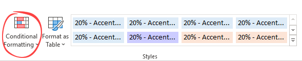
- Click on the Home tab.
- Find the Conditional Formatting icon in the Styles Group.
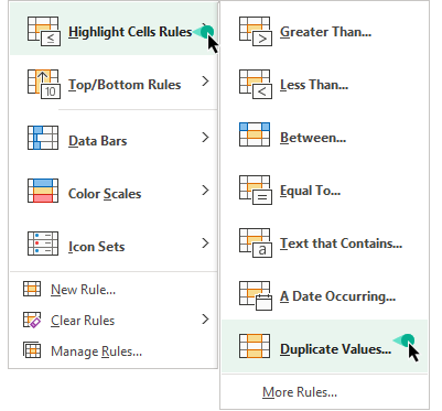
- Click Highlight Cells Rules.
- Choose the ‘Duplicate Values’ command from the list.
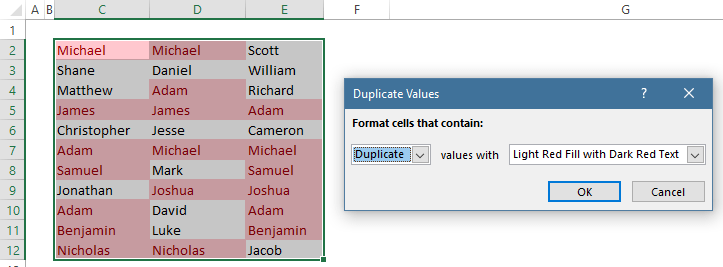
- Select a formatting style.
- Click OK.
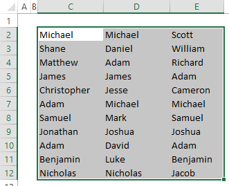
Example
In the example, I’ll select data first; in this case, C2:E12
The next step is to locate the Home Tab. Click on it! Choose the Conditional Formatting icon; you can find it under the Styles Group.
We want to find duplicates, so click Highlight Cells Rules and select the ‘Duplicate Values’ command.
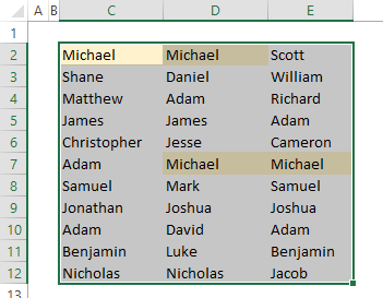
After that, select a formatting style. Click OK. Excel will find the duplicate names in the range and highlight them using the picked color.
Tip: If you want to apply an inverse transformation (for example, find unique values), use the ‘Unique’ option from the list.
How to highlight n occurrences in Excel
You want to find and highlight duplicates using a new rule in the example. Your goal is to find the name with four occurrences.
Select the range C2:E12 and use the formula
=COUNTIF($C$2:$E$12,C2)=4
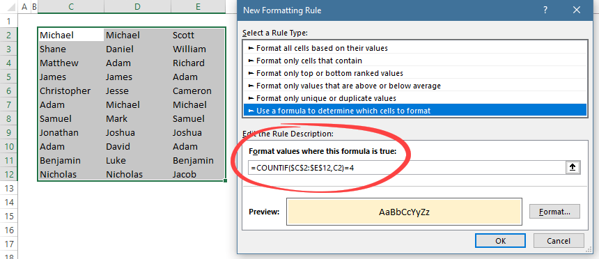
How the formula works:
The =COUNTIF($C$2$:C$12, C2) formula counts the occurrences of records in the range C2:E12 equal to the name in cell C2. Thus, in this example, Michael.
COUNTIF($C$2:$E$12, C2) = 4, so Excel formats cell C2. For example cell C2 contains the formula =COUNTIF($C$2:$E$12,C2)=4, cell C3 =COUNTIF($C$2:$E$12,C3)=4, and so on.
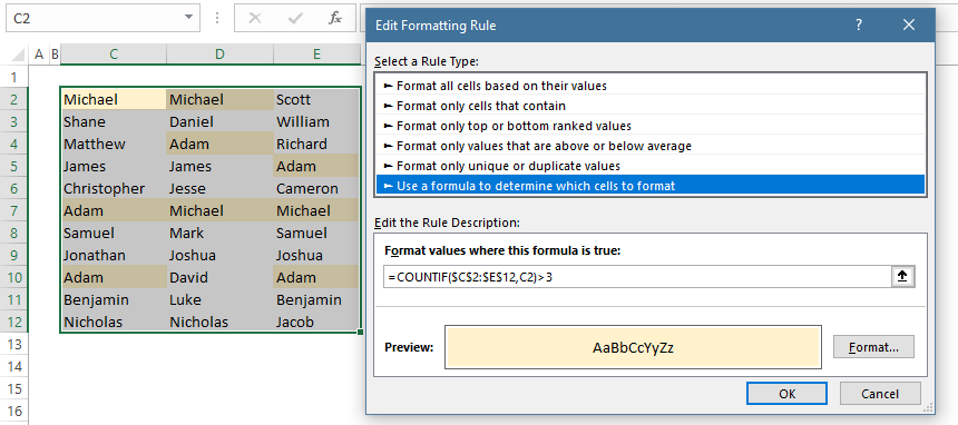
Find duplicates that occur more than n times
If you change the search parameters, you can easily modify the formula. For example, if you want to find and highlight duplicates that occur more than four times, adjust the formula:
For example, =COUNTIF($C$2:$E$12, C1)> 3 will highlight names that occur more than three times.
It’s important to use mixed references. For example, if you use a fixed range, like C2:E12, apply the $ sign, $C$2:$E$12 (absolute references).
The second part of the formula uses relative references.
How to find Duplicate rows in Excel
Steps to find duplicate rows using the COUNTIFS function:
- Select the range H2:H12
- On the Home tab, click Conditional Formatting
- Choose ‘New Rule.’
- In the New Formatting Rule dialog box
- Select the ‘Use a formula to determine which cells to format.’
- Enter the formula: =COUNTIFS(Column1,$H2,Column2,$I2,Column3,$J2)>1
- Select the formatting style and click OK to apply the rule
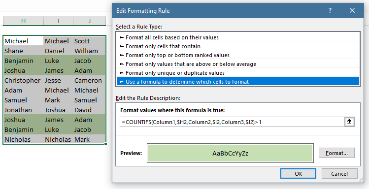
Tip: we strongly recommend you use named ranges instead of cell references.
So, Column 1 refers to the range H2:12, Column 2 refers to I2:12, and Column 3 refers to J2:J12. If you want to remove the duplicated rows quickly, use the Remove Duplicates Tools in Excel.