Learn how to separate names in Excel (first, last, or middle) using regular Excel formulas and advanced functions.
When splitting first and last names in Excel, you can separate names in multiple ways. Simple formulas like LEFT, RIGHT, MID, FIND, or SEARCH can automate the splitting of names, saving time and resources.
You can write custom functions using VBA. These UDFs can manage more advanced tasks and support data cleansing projects. User-defined functions handle exceptions and unique name formats, ensuring effective string manipulations. This article provides a step-by-step guide on separating first and last names using built-in Excel formulas and custom functions.
You can download the practice file containing all examples and source code as usual. Using the training material can save time and reduce the learning curve.
Why is it important to split first and last names in Excel?
Splitting first and last names is key in data handling for easy analysis and sorting. Separating first and last names in different columns in Excel is not just about making your list look straight. It helps make your information clear and useful and your work more efficient.
How to separate names with the Text to Columns feature
Text to columns is a great built-in feature in Excel for splitting names. Let us see the step-by-step guide to extract and separate names in seconds.
Steps to separate names in Excel:
- Select the columns that you want to split.
- On the ribbon, click the “Data” tab.
- Choose the “Text to Columns” command.
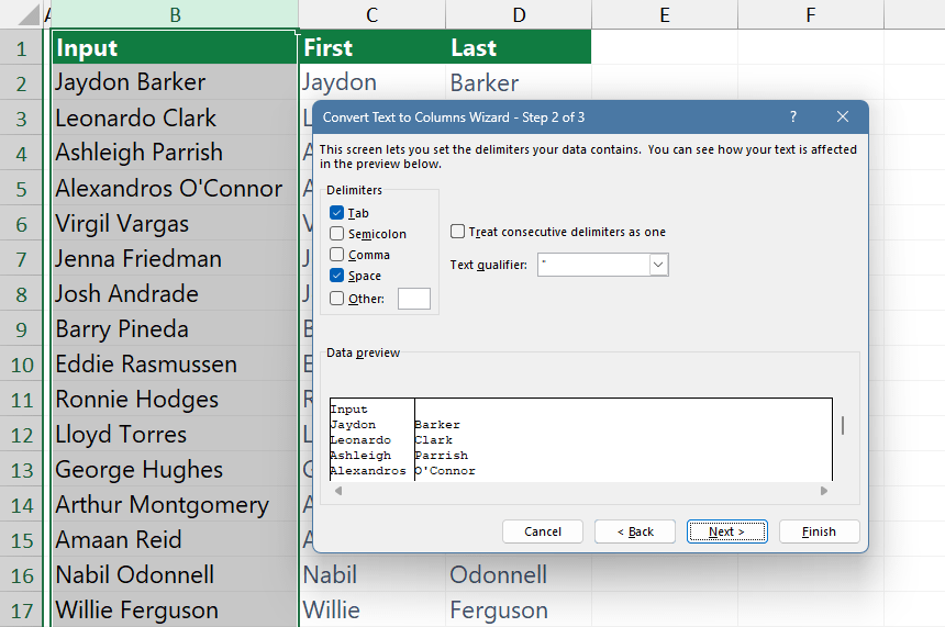
- Select the “Delimited” option.
- Choose the delimiter – for example, a space character or a semicolon.
- Click “Next.”
- Specify the data format.
- Select the location of the output where you want to extract the separated data.
- Click “Finish.”
- Text to Columns separates the first and last names into different cells.
The result looks like the table below:

Note: Clean your data before using this feature. The next chapter will provide effective methods to remove unwanted characters. When the cell includes titles like “Ph.D.”, “Mrs”, or hyphens, you can choose the data cleansing method. If you are a beginner user, apply the “Find and Replace functions”.
Dealing with hyphens and suffixes
It is essential to clean data before separating first and last names in Excel; consistent data is critical for analysis. However, it is not always an easy process to separate names in Excel. Instead of using the time-consuming “Search and Replace” function, apply a specific function to remove prefixes, initials, suffixes, and hyphens.
The TEXTCLEAN function is a custom User-Defined Function (UDF) in Excel designed to sanitize a string (typically a name) by removing a set of unwanted characters. This function can be beneficial in data cleaning, mainly when your dataset contains unwanted characters, typographical errors, or symbols. These symbols can affect your formulas and analyses.
Syntax:
=TEXTCLEAN(cell, unwanted_chars)
Arguments:
- “Rng” takes the cell reference containing the text you want to clean. The function reads the string from this cell.
- “unwanted_chars” is a comma-separated list of characters you want to remove from the cell containing text or names. The function will parse this list and remove all instances of each symbol from the text.

In the example, the range B3:B7 contains names and some unnecessary characters.
Explanation:
- The Split function divides the string into an array based on the delimiter.
- Next, substitute each unwanted character with an empty string.
- Finally, TEXTCLEAN applies the Trim function to clean and extract it without unwanted characters and extra spaces.
The function performs an additional step before returning the final name. After the first cleanup phase, multiple spaces can be left behind. The function uses smart logic and ensures that you have only a single space between the separated names.
Download the Workbook containing the TEXTCLEAN function.
Separate first names using formulas
There are several methods to split the first name; one of the most efficient formulas contains the LEFT and FIND functions. This section will explore the steps to use this formula through examples.
How to separate first names in Excel?
- Select cell D3.
- Type the formula: =LEFT(B3,FIND(” “,B3)-1).
- Press Enter.
- The formula returns the first name.
Generic formula to separate first names:
=LEFT(full_name,FIND(” “,full_name)-1)
In the example, the full name in cell B3 is “John W. Doe”. The goal is to extract and separate the first name into a single cell.
Formula:
=LEFT(B3,FIND(” “,B3)-1)

The formula combines two functions: LEFT and FIND. LEFT extracts a certain number of characters from the left side of a text string. FIND locates a string within another string.
Get the first name using the TEXTLEFT function
Syntax:
=TEXTLEFT(cell, delimiter)
Arguments:
- “txt” refers to the cell range (or the text) from which we want to extract content.
- “delim” is the delimiter defined by a set of characters where the function should stop extracting the text.
- “n” is an optional argument; the default value is 1. The argument defines the number of occurrences of the delimiter.
- “IgnoreCase” is a boolean value. In the case of TRUE, the search for the delimiter is case-insensitive, which means “a” and “A” are considered the same.
=TEXTLEFT(B3,” ”,1)
In the example, you have a text in B3 and want to extract the first name. Use the formula:
Result:

Explanation of parsing logic:
- The function first checks the input text length. If the length is greater than 0, the cell is not empty.
- Within the loop, the InStr function searches for the position of the delimiter in the text. InSrt starts the search after the end of the last found delimiter and checks the comparison type (case-sensitive or not).
- If no delimiter is found, the “delimiter” variable will be 0, and the loop will exit.
- If the “delimiter” is greater than 0 (delimiter was found), the LEFT function extracts characters from the left of the original text until the user-defined delimiter.
Case-sensitivity analysis: First, the function checks the IgnoreCase parameter. If the boolean value is TRUE, the functions use case-insensitive comparison. Otherwise, TEXTLEFT uses the built-in vbBinaryCompare function and applies a case-sensitive comparison.
This function is useful in name-splitting scenarios.
Get last names from the name
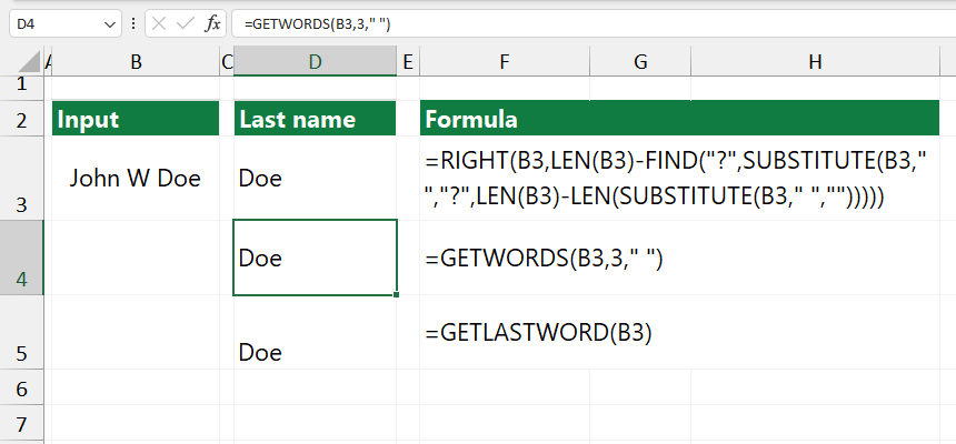
Let us see an example of how to get the last name from a full name using regular Excel text functions. Now you have the full name, “John_ W Doe”, in cell B3, and you want to separate the last name, “Doe”.
Formula to extract the last name from a name:
=RIGHT(cell,LEN(cell)-FIND(“?”,SUBSTITUTE(cell,” “,”?”,LEN(cell)-LEN(SUBSTITUTE(cell,” “,””)))))

Let’s break down the formula step-by-step to understand how it works:
- SUBSTITUTE(cell,” “,”?”, LEN(cell)-LEN(SUBSTITUTE(cell,” “,””))) finds the position of the last space in your text string.
- SUBSTITUTE(cell,” “,””) removes all spaces within your text.
- LEN(cell)-LEN(SUBSTITUTE(cell,” “,””)) calculates the number of spaces in the cell that contain names.
- SUBSTITUTE(cell,” “,”?”,number_of_spaces) replaces the last space in the text with a question mark (“?”)
- FIND(“?”,…) search the “?” position within the text. The formula replaces the “?” character and gets the position where the last word starts.
- LEN(cell) returns the total text length within the cell.
- RIGHT(cell, LEN(cell)-FIND(“?”,…)) extracts a certain number of characters from the right side of the text. It takes the total length of your text. Next, subtract the “?” position to calculate the number of characters it needs to extract. The result is the length of the last word. By subtracting the position of the “?” from the total length, you are left with just the position of the start of the last name to the end of the text, which is the length of the last word.
- RIGHT(cell, number_of_characters) extracts these characters, starting from the right; in other words, separate the last name.
So, if you had a cell that contained the text “John W. Doe”, the formula would replace the last space with a “?”. The result is “John_ W?Doe”. Next, find the position of “?”. Finally, extract “Doe” from the cell using the RIGHT function.
Separate middle names from full name
In the example, you want to get the middle name from the full name. Let us see how to write a formula that uses built-in Excel functions only.
How to extract a middle name from a full name in Excel?
- Select cell B6
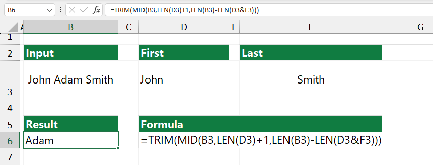
- Type the formula: =TRIM(MID(B3,LEN(D3)+1,LEN(B3)-LEN(D3&F3)))
- Press Enter
- The formula returns the middle name from the full name.
Generic Formula:
=TRIM(MID(full name, LEN(first name)+1,LEN(full name)-LEN(fisrt name&last name)))
Before executing the formula, separate the first and last names using the abovementioned formulas. The MID function starts extracting characters right after “John”. It extracts the number of characters that are left after subtracting the lengths of “John” and “Smith” from “John Adam Smith”. TRIM would clean up unnecessary spaces, returning ‘Adam’ as the final output.
Result:

Take a closer look under the hood:
- MID(full name, LEN(first name)+1, LEN(full name)-LEN(first name&last name)): The MID function is used to extract a specific substring from the ‘full_name’ string, starting at a certain position and extending for a certain number of characters.
- LEN(first_name)+1 calculates and prepares the MID function’s starting position. It finds the length of the first name and adds 1.
- LEN(full name)-LEN(first name&last name) returns the number of characters to extract. It starts by getting the total length of ‘full name’. Next, subtract the combined length of the first name and last name. The ‘&’ character is concatenating first and last names. This subtraction leaves you with the length of the middle name.
- TRIM(…) removes any extra spaces from the text obtained by the MID function and cleans the results by removing leading or trailing spaces.
Related Formulas
- Excel SUBSTRING functions: How to extract text from cell
- How to extract numbers from strings in Excel
- How to extract words from a string in Excel: first, last, or nth
- Regular Expressions in Excel
