Learn how to sum every n rows in Excel using regular functions like SUM and OFFSET. Alternatively, you can apply user-defined functions.
How to sum every n rows in Excel?
Steps to summarize every n rows:
- Open Excel
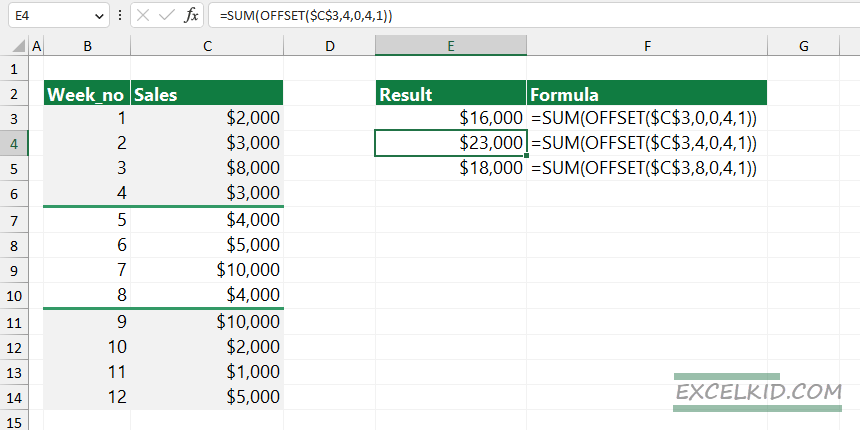
- Enter the formula: =SUM(OFFSET($C$3,0,0,4,1))
- Press Enter
- The formula calculates the sum of the first four rows starting from cell C3.
Explanation
The OFFSET and SUM functions allow you to sum a specified range dynamically. Here’s how the formula works:
- OFFSET($C$3,0,0,4,1): The OFFSET function creates a reference that starts at cell C3.
- $C$3: The starting point for the reference.
- 0 (row_num): Moves zero rows down, keeping the start at C3.
- 0 (col_num): Keeps the reference in the same column as C3.
- 4 (height): Expands the reference to cover the next 4 rows.
- 1 (width): Covers a single column.
- SUM: This function adds the values in the range created by the OFFSET function.

In the example, the formula sums every 4 rows in column C. The first sum will include rows 3 to 6. To sum the next group, adjust the row offset (e.g., =SUM(OFFSET($C$3,4,0,4,1)) for rows 7 to 10). This method allows for flexible summing based on different row groupings, controlled by the height argument in the OFFSET function.
How to sum every n rows using a UDF
You can use user-defined functions to speed up the work:
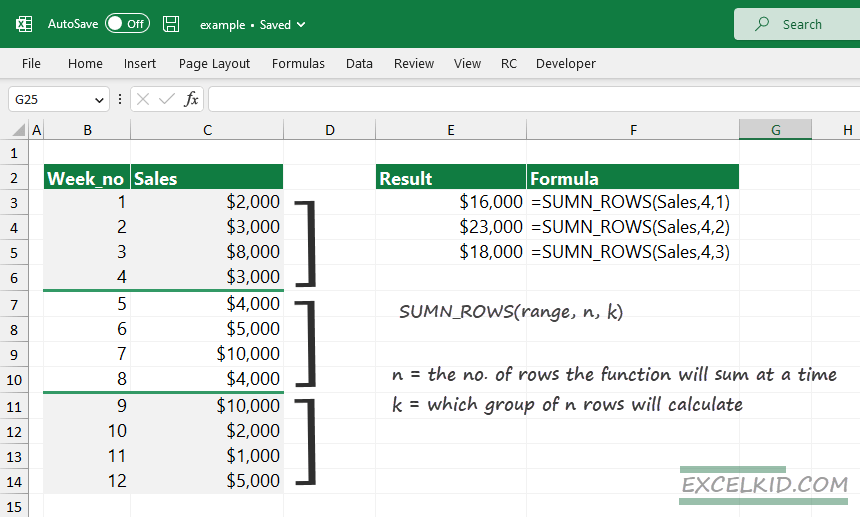
- Enter SUMN_ROWS(C3:C14, 4,2) function
- Select the range: C3:C14
- Add how many cells you want to summarize (4)
- Set which group of n rows will calculate (2)
- The function returns the sum of every n rows
Function arguments:
- rng: The range to be summed.
- n: The number of rows to sum together at a time.
- k: The index of the group of rows to sum.
The point is that you specify the group of cells you want to sum. You also add two arguments, n, and k, and both numbers are integers. The first argument (n) controls the number of rows the SUMN_ROWS will use – the third argument (k) controls which group of n rows will summarize.

In the example, you want to sum every n rows. Take a look at the picture below! First, select the range C3:C14 and add a descriptive name for a range, for example, “Sales”. You can add a name to a range by clicking the name box.
If you want to sum the sales between Week 5 and Week 8, use the following formula:
=SUMN_ROWS(Sales, 4, 2)
First, you need to add the range. Select cell C3:C14. We find a group that contains 4 records, so add “4” as a second argument. To get the sum of Sales between the 4th and 8th week, you need to use the second group, C7:C10; the third argument is “2”.
=SUMN_ROWS(Sales, 4, 2)
=SUM(C7:C10) = 4000 + 5000 + 10000 + 4000
=23000
You can paste the code below to use the function.
Function SUMN_ROWS(rng As Range, n As Integer, k As Integer) As Double
    Dim startRow As Integer
    Dim endRow As Integer

    ' Determine the starting and ending row
    startRow = (k - 1) * n + 1
    endRow = k * n

    ' Check if the specified row group is within the range
    If startRow > rng.Rows.Count Then
        SUMN_ROWS = 0
        Exit Function
    End If

    If endRow > rng.Rows.Count Then
        endRow = rng.Rows.Count
    End If

    ' Sum the selected group of rows
    SUMN_ROWS = Application.WorksheetFunction.Sum(rng.Rows(startRow & ":" & endRow).SpecialCells(xlCellTypeConstants))
End Function
Related formulas
- How to sum the top N values in Excel?
- Sum values in a range between two numbers
- Count cells between two numbers
- Sum bottom n values in a range