This tutorial shows how to create an IF formula with Boolean logic to sum values based on multiple conditions.
How to use an IF formula with Boolean logic?
Here are the steps to sum quantities with multiple conditions using Boolean logic in Excel:
- Open Excel
- Type =SUM(IF((product=”Apple”)*(color=”Blue”)*(quantity>40), quantity))
- Press Enter
- The formula will return the sum of quantities where the product is “Apple,” the color is “Blue,” and the quantity is greater than 40.
Example
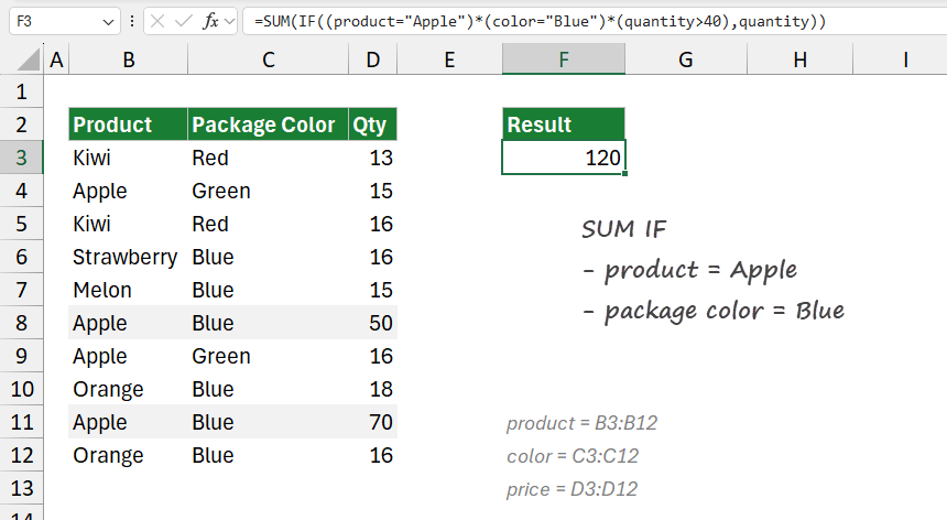
First, create three named ranges:
- product = B3:B12
- color = C3:C12
- quantity = D3:D12
The goal is, to sum up the quantity values for entries that meet three specific conditions:
- product=”Apple”: Only considers rows where the product is “Apple.”
- color=”Blue”: Only includes rows where the package color is “Blue.”
- quantity>40: Only includes rows where the quantity is greater than 40.
Formula:
=SUM(IF((product=”Apple”) * (color=”Blue”) * (quantity>40), quantity))

The result is 120.
Explanation
The first step is to use a logical test.
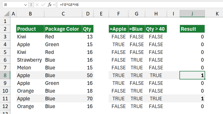
- Apply multiple conditions: (product=”Apple”) * (color=”Blue”) * (quantity>40): Each condition here returns either TRUE or FALSE. When multiplied together, only rows where all three conditions are TRUE will produce a 1 (since TRUE * TRUE * TRUE = 1). If any condition is FALSE, the result will be 0, excluding that row from the sum.
- IF and SUM Functions: IF(…, quantity): For rows where the logical test returns 1, the IF function includes the quantity in the result; otherwise, it returns 0. Finally, SUM(…) adds up all the quantity values that met the conditions.

Use the multiplication sign to convert boolean TRUE and FALSE values into 0s or 1s. As you see, only two rows meet the criteria.
SUMIFS function
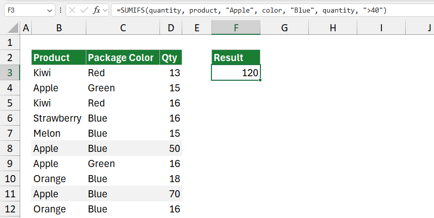
Here is an alternative if you want to avoid the array formula requirement. The formula calculates the total quantity values for rows where three specific conditions are met.
Formula:
=SUMIFS(quantity, product, “Apple”, color, “Blue”, quantity, “>40”)

Using FILTER and SUM
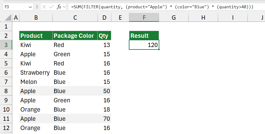
You can apply multiple conditions using a formula based on the FILTER and SUM functions.
Formula:
=SUM(FILTER(quantity, (product=”Apple”) * (color=”Blue”) * (quantity>40)))

You can download the Workbook, which contains the sample data and the formulas.