The Excel IFS function performs multiple logical tests and allows you to create shorter, easy-to-read formulas.
In this tutorial – from the ground up, we will show you how the function works through practical examples.
What is the IFS function in Excel?
Excel IFS function can run multiple tests and return the user-defined value when the first TRUE result is found. To create a more user-friendly formula, use the IFS function to test multiple conditions without struggling with the nested IF statements.
The IFS function uses the following logic: the function evaluates the first condition. If the result is FALSE, it jumps to the next condition and re-evaluates the test using the right-to-left direction. Once the first TRUE output is found, the function returns with the value of the corresponding “value_if_true” argument.
IFS supports a maximum of 127 conditions and argument pairs.
The function is available in Excel for Microsoft 365, Excel 2021, and Excel 2019.
Syntax and arguments, structure
Syntax:
=IFS(test1, value_if_true1, [test2, value_if_true2], …)
Arguments:
- test1 – the first logical test.
- value1 – the result is when test1 is TRUE.
- test2, value2 – [optional arguments] is the second test/value pair.
Explanation:
Inside the IFS formula, you will find pairs, like in the example below. It is worth splitting the formula into test/value pairs. Press the Alt + Enter keyboard shortcut to create the right structure.

IFS Function Examples
This section will provide useful examples and formulas based on the IFS function.
Example #1 – Test scores, lowest to highest
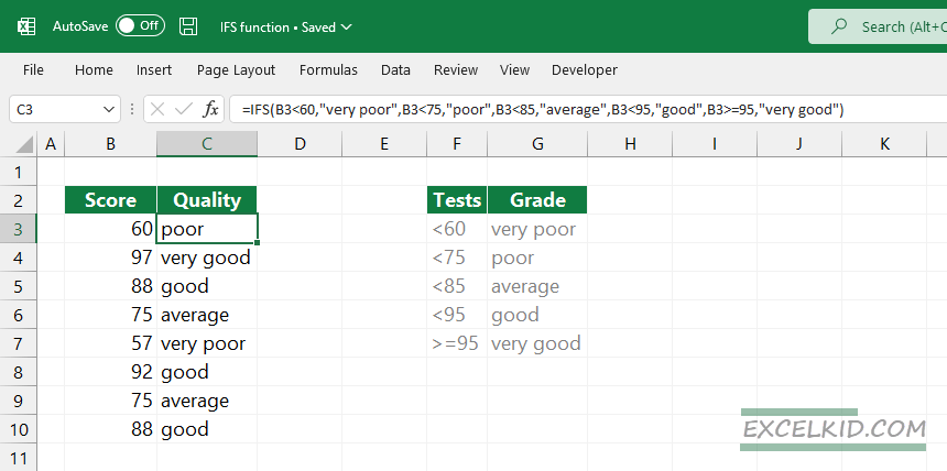
In the example, we’ll explain how the order of the arguments works if we use the lowest to the highest rating.
Conditions are the following:
- if the score is less than 60, the result is “very poor”,
- scores between 60 and 75 are “poor”,
- between 75 and 80, we use the “average” flag,
- between 85 and 95, the result is “good”,
- if the score is greater than or equal to 95, the rating is “very good”.
To assign the values to rating using IFS, here are the conditions:
- <60 = very poor
- <75 = poor
- <85 = average
- <95 = good
- >= 95 = very good

Enter the conditions from left to right in ascending order; use the lowest score first. The quality associated with the first test to return TRUE is returned.
=IFS(B3<60,"very poor",B3<75,"poor",B3<85,"average",B3<90,"good",B3>=90,"very good")Example #2 – Test scores, highest to lowest
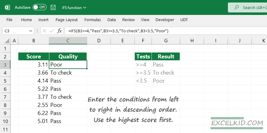
We will use the second example’s inverse rating system, a quality test. The conditions are as follows: if the value in B2 is greater than or equal to 4, the result will be “Pass”. If the value is less than 4 but greater than or equal to 3.5, the status is “To check”. Finally, if the value is less than 3.5, the formula will return “Poor”.
Create a formula and enter the conditions from left to right in descending order. Use the highest score first.

=IFS(B3>=4,"Pass",B3>=3.5,"To check",B3<3.5,"Poor")IFS function: Error handling (if an exact match is not found)
In the last example, we explain what will happen (and how to fix it) if none of the tests returns the TRUE result.
Excel IFS function does not support a native error-handling argument when all conditions are the FALSE results. The good news is that we can add TRUE as a default value at the end of the formula.
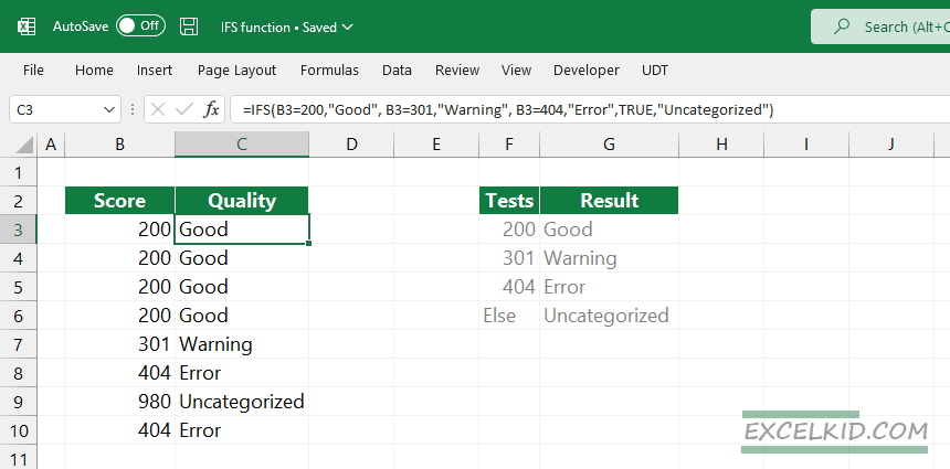
In the example below, we will use three possible outputs. If the value is 200, the formula returns with “Good”. Furthermore, the value is “Warning” if it equals 301. The result is an “Error” if the value is 404. In any other cases, we use the “uncategorized” output. To do that, enter the TRUE as the last test. Finally, we create a user-defined output in case no match is found.
=IFS(B3=200,"Good", B3=301,"Warning", B3=404,"Error",TRUE,"Uncategorized")
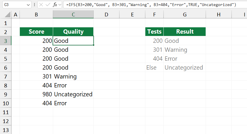
The IFS formula splits the list into four categories.
Differences between IFS and SWITCH functions
The SWITCH and IFS functions enable using more than one condition in a single formula. Both functions are a really good replacement for the old IF function. Both formulas remain easy to read even if you are using multiple conditions. That’s what matters!
Sometimes, the SWITCH function provides better usability because you can use the expression once in a formula. Furthermore, SWITCH has a native argument for managing the default value. The main problem is that you can not use logical operators as usual, and the function can handle only exact matches.
Things to remember
- IFS function does not provide a default value if all tests return FALSE.
- To create a default value, use TRUE as the last logical test and add a custom value for error-handling purposes.
- IFS return a #VALUE! Error if the test is not TRUE or FALSE.
- If all logical test returns FALSE, use a custom TRUE value; else, IFS will return the #N/A error
