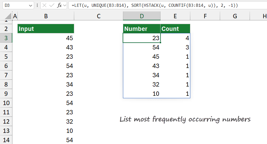
To list the most frequently occurring numbers in a column, use a formula based on the LET, UNIQUE, SORT, HSTACK, and COUNTIF functions.
How to list the most frequently occurring numbers in Excel?
Steps to get the most frequently occurring numbers in a range:
- Select cell D3.
- Type =LET(u, UNIQUE(B3:B12), SORT(HSTACK(u, COUNTIF(B3:B12, u)), 2, -1))
- Press Enter.
- The formula lists all unique elements along with their occurrence counts.
Example
In the example, we have numbers in the range B3:B14. The goal is to create a list of unique numbers sorted by their frequency in descending order.
Formula:
=LET(u, UNIQUE(B3:B12), SORT(HSTACK(u, COUNTIF(B3:B12, u)), 2, -1))

The result looks great; now we have a list that contains the most frequently occurring numbers in an ordered list.
Explanation
Take a closer look at the formula:
LET(u, UNIQUE(B3:B14), …)
The LET function in Excel allows you to assign names to expressions or values and then use these names within the formula, making it easier to read and more efficient by avoiding repeated calculations. Here, LET assigns the name u to the result of UNIQUE(B3:B14).
UNIQUE(B3:B14)
UNIQUE extracts a list of unique values from the range B3:B14 containing the numbers. For example, if B3:B14 has values like {45, 43, 23, 54, 23, 34, 23, 32, 10, 54, 23, 10}, UNIQUE(B3:B14) returns {45, 43, 23, 54, 34, 32, 10}. The unique list of numbers is now assigned to the variable “u”, which will be used in subsequent calculations.
COUNTIF(B3:B14, u)
COUNTIF counts how many times each unique value (in u) appears in the original range B3:B14. Since “u” is an array of unique numbers, COUNTIF(B3:B14, u) generates a corresponding array with the counts for each number in u. For example, if “u” is {45, 43, 23, 54, 34, 32, 10}, COUNTIF(B3:B14, u) might return {1, 1, 4, 3, 1, 1, 1}, indicating that 45 appears once, 43 once, 23 four times, and so on.
HSTACK(u, COUNTIF(B3:B14, u))
HSTACK horizontally stacks two arrays, creating a two-column array. The first column is u (the unique numbers from B3:B14). The second column is the counts of each number, as calculated by COUNTIF. The resulting array might look like this: {23, 4; 54, 3; 45, 1; 43, 1; 34, 1; 32, 1; 10, 1}
SORT(…, 2, -1)
The SORT function sorts the array generated by HSTACK in descending order based on the second column (the counts). The 2 argument specifies that sorting should be based on the second column. The -1 argument indicates descending order.
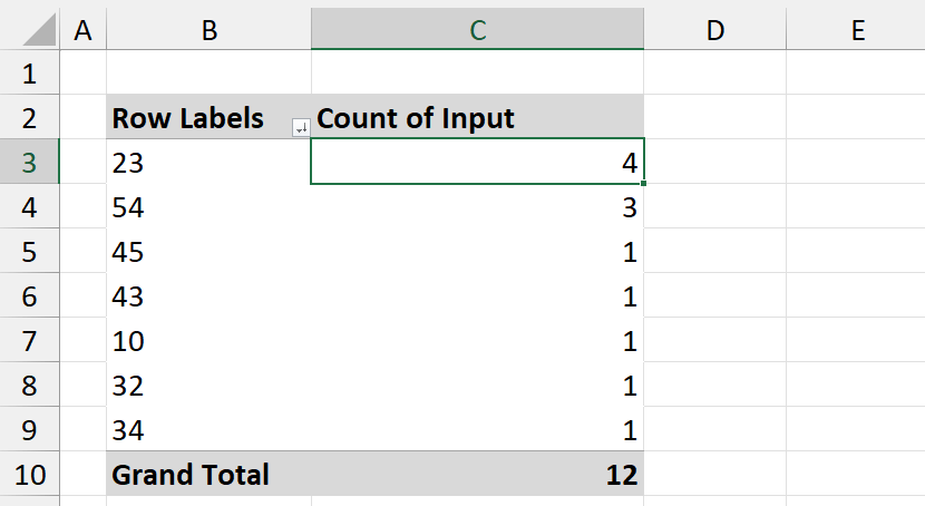
Workaround with Pivot tables
Creating a Pivot Table on the B3:B14 range can achieve the result without formulas. Set the values to “Count” and sort the counts in descending order.
