To match the first error in a range in Excel, you can apply a formula based on the XMATCH, TRUE, and ISERROR functions.
How to match the first error in Excel?
Here are the steps to match the first error in a range in Excel:
- Open Excel.
- Type =XMATCH(TRUE, ISERROR(A1:A10), 0)
- Press Enter.
- The formula returns the position of the first error in the specified range A1:A10.
Example
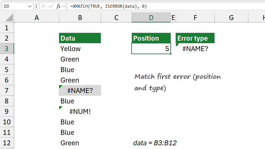
In the example, the data is in the range B3:B12. First, select the data and create a named range, “data.”
Formula:
=XMATCH(TRUE, ISERROR(data), 0)
Result:

The formula =XMATCH(TRUE, ISERROR(data), 0) is designed to find the first cell in the range B3:B12 that contains an error.
Explanation
Evaluate the formula from the inside out.
ISERROR(A1:A10)
The ISERROR function checks each cell in the range B3:B12 to see if it contains an error. ISERROR returns TRUE for any cell with errors (such as #DIV/0!, #N/A, #VALUE!, etc.) and FALSE for cells without errors. As a result, ISERROR(data) produces an array of TRUE and FALSE values corresponding to each cell in the range.
In the example, the array might look like this: {FALSE, FALSE, FALSE, FALSE, TRUE, FALSE, TRUE, FALSE, FALSE, FALSE}.
XMATCH(TRUE, ISERROR(A1:A10), 0)
The XMATCH function searches for a specific value (in this case, TRUE) within a range or array.
- The first argument, TRUE, is the value XMATCH is looking for. Here, we’re looking for the first TRUE value, which indicates the first error in the range.
- The second argument, ISERROR(data), is the array that XMATCH will search within. This is the array of TRUE and FALSE values generated by ISERROR.
- The third argument, 0, specifies an exact match. XMATCH will find the first occurrence of TRUE in the array, corresponding to the first error in the range B3:B12. If TRUE is found, XMATCH returns the position (relative to the array B3:B12) of the first TRUE in the array, corresponding to the position of the first error in the range. For example, if the first error is in B7, XMATCH would return 5, as B7 is the fifth position in the range B3:B12.
The formula returns a number that represents the position of the first cell with an error in B3:B12. If no errors exist in the range, XMATCH will return an #N/A error, as TRUE is not found in the array.
How to identify the type of the first error in a range?
- Open Excel.
- Type =XLOOKUP(TRUE, ISERROR(A1:A10), A1:A10)
- Press Enter.
- The formula returns the first error type in the specified range A1:A10.
Example
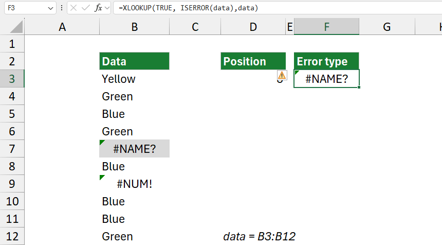
In the example, the goal is to identify the first error type in the selected range.
Formula:
=XLOOKUP(TRUE, ISERROR(data),data)

Take a closer look at the XLOOKUP function:
XLOOKUP(TRUE, ISERROR(data), data): XLOOKUP searches for a specific value (in this case, TRUE) within a lookup array and returns a corresponding value from a result array.
- The first argument, TRUE, is the value XLOOKUP seeks in the lookup array.
- The second argument, ISERROR(data), is the lookup array where XLOOKUP searches for TRUE. This array contains TRUE for cells with errors and FALSE for cells without errors.
- The third argument, data, is the result array. When XLOOKUP finds the first TRUE in the lookup array, it returns the corresponding value from the data array. This means that XLOOKUP will return the first cell in data that contains an error.