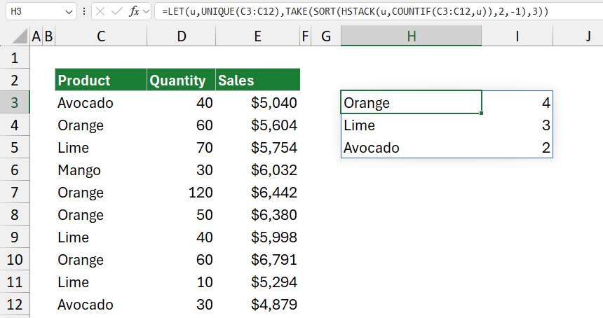
To list the most common text values in a column or a row, you can use a formula using the LET, UNIQUE, SORT, HSTACK, and COUNTIF functions.
How to find the most common text values in Excel?
Steps to find the most common text values in a column or a row:
- Open Excel.
- Type =LET(u,UNIQUE(C3:C12),TAKE(SORT(HSTACK(u,COUNTIF(C3:C12,u)),2,-1),3))
- Press Enter.
- The formula returns the top 3 most frequent products with their counts.
Example
This formula counts how often each unique product appears in C3:C12, sorts the products by frequency in descending order, and displays the top 3 results.
Formula:
=LET(u,UNIQUE(C3:C12),TAKE(SORT(HSTACK(u,COUNTIF(C3:C12,u)),2,-1),3))

Now, evaluate the formula from the inside out.
Explanation
LET Function:
LET allows us to define variables within the formula to simplify it and improve its readability. Here, u represents the list of unique items in C3:C12.
UNIQUE(C3):
The UNIQUE function extracts all unique product names from the range C3:C12. For instance, if C3:C12 contains {Avocado, Orange, Lime, Mango, Orange, Orange, Lime, Orange, Lime, Avocado}, UNIQUE(C3:C12) will return {“Avocado”, “Orange”, “Lime”, “Mango”}, which represents each distinct product name in the list.
COUNTIF(C3, u):
COUNTIF(C3:C12, u) counts how often each unique product appears in C3:C12.
Since “u” is an array of unique product names, COUNTIF evaluates each product individually and returns an array of counts corresponding to each unique product. For example, it might return {2, 4, 3, 1} if Avocado appears twice, Orange four times, Lime three times, and Mango once.
HSTACK(u, COUNTIF(C3, u)):
HSTACK horizontally stacks the unique products array (u) with their counts, creating a two-column array.
The result might look like this: {{“Avocado”, 2}; {“Orange”, 4}; {“Lime”, 3}; {“Mango”, 1}}.
SORT(HSTACK(u, COUNTIF(C3, u)), 2, -1):
SORT organizes the array by the second column (the count) in descending order (-1). This sorting step ensures that products with the highest counts appear at the top of the list. The sorted array might look like this: {{“Orange”, 4}; {“Lime”, 3}; {“Avocado”, 2}; {“Mango”, 1}}.
TAKE(SORT(…), 3):
TAKE extracts the top 3 rows from the sorted array. This ensures that only the three most frequent products are displayed. Based on the previous example, TAKE would return {{“Orange”, 4}; {“Lime”, 3}; {“Avocado”, 2}}.
This formula counts each unique product in C3:C12, sorts them by frequency in descending order, and displays the top 3 most frequent products with their counts.
Workaround with SORTBY and UNIQUE
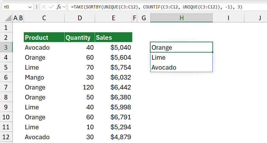
You can apply a formula that directly sorts the unique values based on their frequency without needing HSTACK.
=TAKE(SORTBY(UNIQUE(C3:C12), COUNTIF(C3:C12, UNIQUE(C3:C12)), -1), 3)

An alternative approach could use INDEX, MATCH, and LARGE functions to retrieve top frequencies manually, though it would be more complex and less dynamic than using LET with dynamic arrays.