In this tutorial, you will learn how to return the nth value in a row using the CHOOSECOLS function in Excel.
How to return the nth value in a row?
Steps to get the nth value in a row:
- Open Excel
- Type =CHOOSECOLS(D2:I2, 4)
- Press Enter
- The formula returns the 4th value in the row
CHOOSECOLS Formula
The CHOOSECOLS function returns the specified columns from an array. The function is available in Excel for Microsoft 365. With a little trick (using only the required arguments), you can use the function to extract the nth value in a row. Swiss-knife.
Syntax:
=CHOOSECOLS(array, col_num1, [col_num2])
Arguments:
The function uses two required arguments, but you can add additional columns as optional argument(s).
- array: the array where you find the nth value (row)
- col_num1: an integer value, it represents the nth value
- col_num2: optional argument
Example
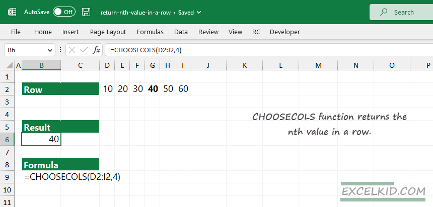
In the example, you want to return the 4th value in a selected range, D2:I2.
Formula:
=CHOOSECOLS(D2:I2, 4)

Evaluate the formula: First, select the range (row) where you want to find the nth value, in this case, D2:I2. After that, add an integer as a second argument; we find the 4th value in the given row, so add “4” as a col_num1 argument.
Workaround with the OFFSET function
You can use the OFFSET function if you are working with an earlier version of Excel (for example, Excel 2010, Excel 2013, or Excel 2016).
Formula:
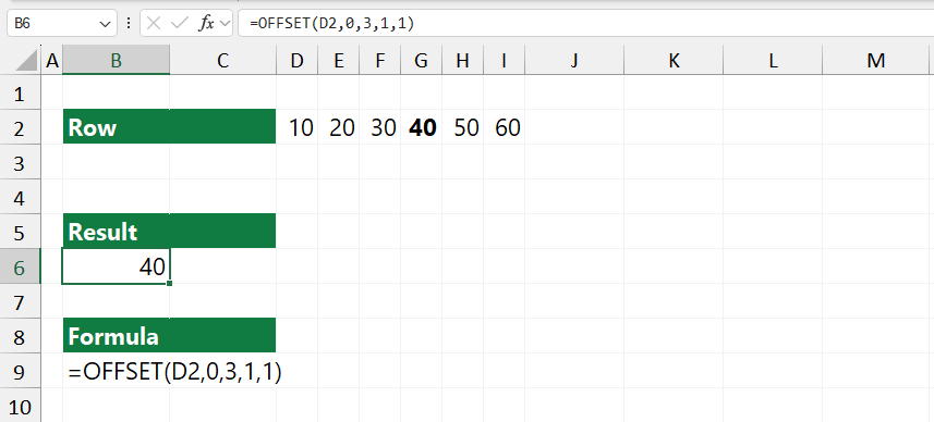
=OFFSET(D2,0,3,1,1) = 40

Explanation: The OFFSET function works like a “moving range” that you can use to return different parts of the Worksheet, in this case, a single cell. The reference is the starting point, cell D2. We find the nth value in the same column, so the second argument is 0. To get the fourth value, we must move the range right with 3 cells: the third argument is 3. The fourth and fifth arguments are 1 since we want to extract a single value.
The result is the same.
Related Formulas
- SUM every nth column
- How to get the nth value in a column?
- SUM Top n values
- How to sum the last n rows?
- SUM every nth row
- SUM last n columns