This tutorial will show you how to split dimensions into two parts and extract the left and right dimensions into separate values.
The example contains a list of custom text dimensions as raw data. Our goal is to split the original text into two parts. First, we’ll use formulas based on regular Excel functions and -as usual- user-defined functions.
How to Split dimensions into two parts
Steps to split dimensions into two different parts:
- Open Excel.
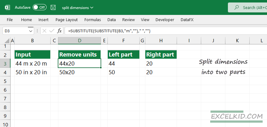
- Type =SUBSTITUTE(SUBSTITUTE(B3,”m”,””),” “,””)
- Press Enter.
- The formula splits the dimensions into two parts.
Explanation
Extracting the numbers from the cell is not easy, so we’ll show you two different methods. Extracting individual dimensions from a text can be performed with built-in Excel formulas that combine several text manipulation functions. Our worksheet contains text dimensions (for example, “10 m x 85 m”). The dimensions include both the “m” unit and space characters (” “).
In a nutshell, we’ll use the steps below:
- Remove the unwanted characters (spaces) from the original string.
- Remove the units
- Extract the left part of the expression
- Get the right part of the expression
We’ll apply a nested formula using the SUBSTITUTE function.
=SUBSTITUTE(SUBSTITUTE(B3,”m”,””),” “,””)
Check the result in cell D3. Then, using the formula mentioned earlier, we can remove the unnecessary spaces and units. This nested functions-based formula leaves the numeric parts of the original text. The inner section strips the “m” character:
=SUBSTITUTE(B3,”m”,””)
The outer section of the formula eliminates unnecessary spaces.
=SUBSTITUTE(SUBSTITUTE(B3,”m”,””),” “,””)
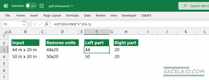
We need only the separator character because, with its help, we can extract the left and the right sections. The formula in cell F3:
=LEFT(B3,FIND(“x”,B3)-1)
And voila, the result is the left numeric part of the original text.
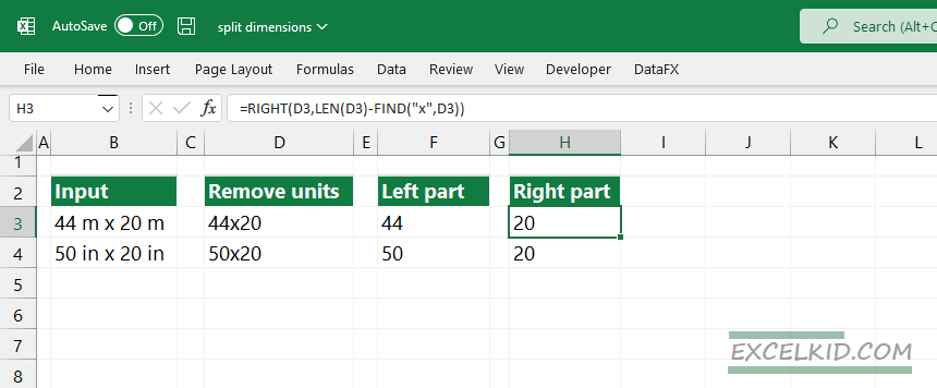
Use the formula below to extract the dimension from the right:
=RIGHT(D3,LEN(D3)-FIND(“x”,D3))
Okay, take a look at the other solution!
Using the SUBSTRING function
The best way to normalize text is by using the SUBSTRING function. Use our free function library to push the limits in Excel.
Formula:
=CONCAT(Substring1, Substring2, Substring3)
We already know how the CONCAT function works. The Substring function returns the nth element of the text string, where a specified separator character separates the parts.
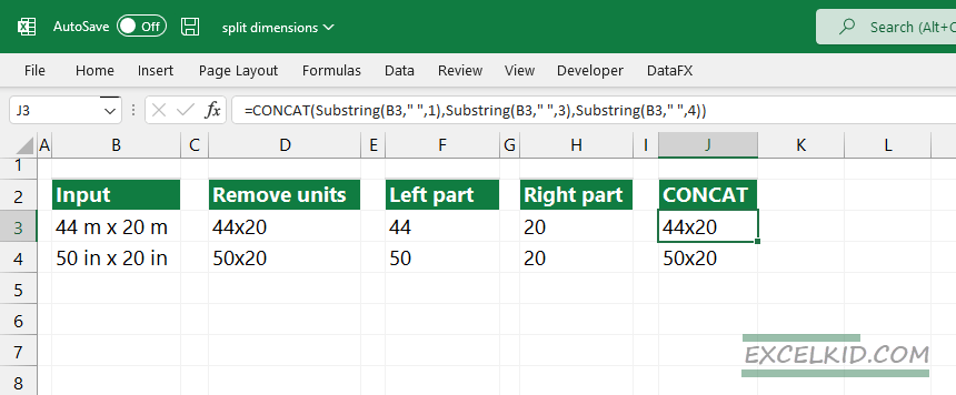
First, combining three substring functions gets the dimensions and the separator character.
- =Substring(B3,” “,1) = 44
- =Substring(B3,” “,3) = x
- =Substring(B3,” “,4) = 20
Finally, join the substrings using the CONCAT function:
=CONCAT(Substring(B3,” “,1),Substring(B3,” “,3),Substring(B3,” “,4))
From now on, apply the LEFT and RIGHT functions to split dimensions into two parts.
Related Formulas and Examples
- Get the first word from some text
- Get the last word from a text string
- Split text with delimiter
- Abbreviate names