To sum the first n matching values in a range in Excel, you can use a formula based on the SUM, TAKE, and FILTER functions.
How to sum first n matching values in Excel
Here are the steps to sum the first n matching values in Excel:
- Open Excel.
- Type =SUM(TAKE(FILTER(range, criteria), n)).
- Press Enter.
- The formula will return the sum of the first n values that meet the specified criteria.
Explanation
The formula =SUM(TAKE(FILTER(range, criteria), n)) calculates the sum of the top “n” values that meet specific criteria within a given range.
Evaluate the formula from the inside out:
- FILTER(range, criteria): The FILTER function examines the range and extracts only the values that meet the specified criteria. This step creates a subset of values based on the condition provided. For example, if the range is a list of numbers and the criteria specify that only values greater than a certain threshold are included, this will produce an array containing only those values that satisfy the criteria.
- TAKE(filtered_array, n): Once FILTER generates a list of values, TAKE extracts the first “n” values from this filtered list. Using TAKE on data sorted in a certain way (e.g., descending order) would give you the “n” largest values meeting the criteria.
- SUM: The SUM function then adds up these extracted “n” values, giving you the total of the specified items that met the initial criteria.
Note: Without sorting, it simply picks the first “n” entries in the order they appear after filtering.
Example
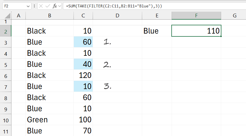
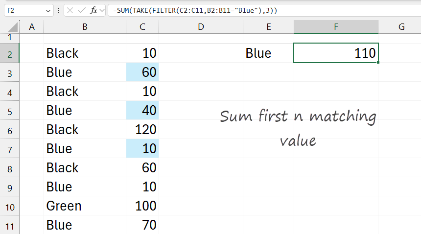
Suppose you have data in a range and want to sum up the top 5 sales values over a certain threshold (like if the color is blue). The following formula sets up criteria to filter for names = “Blue” and specifies n as 3.

Formula:
=SUM(TAKE(FILTER(C2:C11,B2:B11=”Blue”),3))
How the dynamic array formula works:
First, the FILTER(C2:C11, B2:B11=”Blue”) scans through the range B2:B11 to identify cells that match the criteria (=”Blue”). For every cell in B2:B11 that contains “Blue,” the corresponding value from C2:C11 is included in the result.
In this case, the FILTER function returns an array of values from column C, where column B is “Blue.” The resulting array is {60, 40, 10, 10, 70}.
The TAKE function takes only the first n elements from the filtered array. Here, n is 3. From the filtered array {60, 40, 10, 10, 70}, TAKE returns the first three values: {60, 40, 10}.
The formula calculates and returns 110, the sum of the first three “Blue” values from the specified range. If you want to learn all about Excel formulas, check this guide.
