To sum the last N rows in a range, you can use the SUM function with the TAKE function or apply a workaround using the OFFSET function.
How to sum the last n rows in Excel?
- Open Excel
- Type =SUM(TAKE(A1:D20, -n))
- Press Enter
- The formula returns the last n rows.
Example
In the example, the TAKE function allows you to quickly sum the last N rows from a specific range of cells. The function supports dynamic data analysis.
Let’s see the key steps and an explanation of how the function works:

Formula:
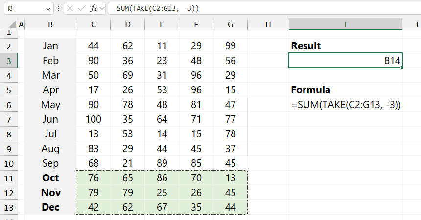
=SUM(TAKE(C2:G13, -3))
Evaluate the formula from the inside out:
- First, TAKE(C2:G13, -3) extracts the last three rows of the specified range. The first argument (C2:G13) is the data range. The second argument (-3) specifies the number of rows from the bottom to take. A negative number selects rows from the bottom, while a positive number would take rows from the top.
- After that, the SUM function adds up the values returned by the TAKE function, providing the total of the last N rows. In this example, the last three rows (October, November, and December) are summed, returning a result of 814.
OFFSET Function
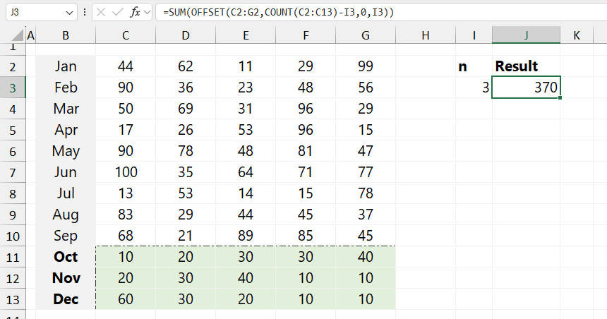
Okay, here is a workaround with the OFFSET function. The goal is the same as the previous example: summarize the last three rows. This function returns a range of cells with a specified number of rows and columns away from a reference point.
Formula:
=SUM(OFFSET(C2:G2,COUNT(C2:C13)-I3,0,I3))
The formula =SUM(OFFSET(C2:G2, COUNT(C2:C13) – I3, 0, I3)) calculates the sum of a specified number of rows from a range, based on certain conditions.
Here’s a step-by-step breakdown:

Explanation:
- COUNT(C2): This part of the formula counts the non-empty cells within the range C2:C13. This count determines how many rows contain data, finding the “end” row for data selection.
- COUNT(C2) – I3: Here, the result of the count is reduced by the value in cell I3. This adjustment specifies the starting point of the range to be summed, effectively “moving up” by I3 rows from the last data row.
- OFFSET(C2, COUNT(C2) – I3, 0, I3): The OFFSET function now uses the adjusted row position:
- C2:G2 is the starting range.
- COUNT(C2:C13) – I3 shifts the starting row down to the target row.
- 0 keeps the column unchanged.
- I3 specifies the height (number of rows) for the range to sum.
- This creates a dynamic range based on the count and value of I3.
- SUM(…): Finally, SUM adds up the values in the defined dynamic range.
Related Formulas
- Return the Nth Value in a Row
- SUM every nth row
- Get the nth value in a column
- Lookup and return the nth value
- SUM last n columns
- SUM every n rows