Learn how to use dynamic color ranking in Excel using conditional formatting and RANK function. In this article, we will discover how to apply the Rank function in Excel and where we need to use it in data.
Use the RANK formula to return the ranking of any number in the data. Mostly we use the rank formula to show the ranking of products, sales, etc.
We’ll apply two easy steps. As first, we’ll use the rank function to determine the sorting order (ranking).
After that, we’ll show you how to highlight the top five products using the most useful Excel built-in tool, conditional formatting.
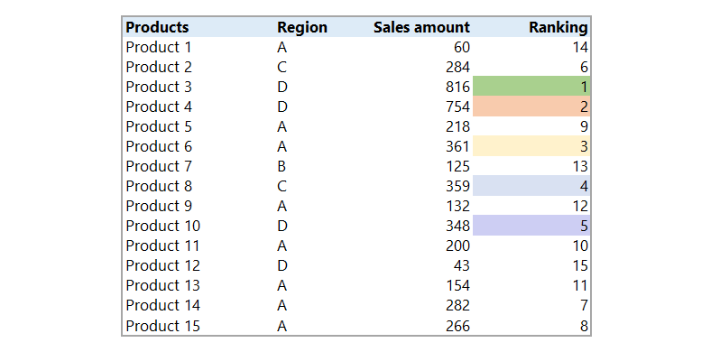
Let’s see the final result below. For better readability, we recommend using different colors for each competitor.
How to use the Excel RANK function
The Excel RANK function returns the rank of a number within a set of numbers, it is a built-in statistical function in Excel.
The syntax is simple:
RANK( number, array, [order] )Just a few words about the parameters. We need only three arguments:
- The number to find the rank for
- A range of numbers that we use for rankings
- Order is an optional parameter to specify how to rank the given numbers.
The Color ranking method – Step by step Tutorial
Step 1: To rank the data quickly, select cell E3 and enter the formula below:
=RANK(D3,$D$3:$D$17,0)Now copy the formula through the given range.
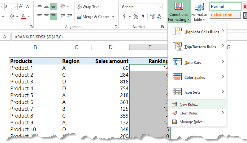
Step 2: Select the range which contains ranks. In this case, select range E3:E17.
Navigate to the Ribbon. On the Home tab, click Home, Conditional Formatting , and choose New Rule.
Step 3: A New Formatting Rule dialogue box will appear.
Select a rule type from the list.
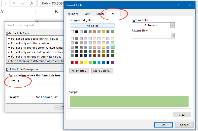
In this example, select the ‘Use a formula to determine which cells to format’.
Enter =$E3=1 into the formula bar.
Click Format and the Format Cells dialogue box will appear. Under the Fill tab, select your preferred color for the top1 result.
Step 4: Click OK to leave the Format Cells dialogue box.
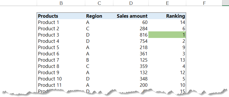
Finally, click OK to apply the new rule. The top 1 product will be highlighted with your selected color.
Step 5: To get the second and the third position, we need to repeat steps 3 and step 4 to highlight the results between 2 and 5.
You need to apply a small modification regarding the formula.
Use
- =$E3=2 for the second,
- =$E3=3 for the third,
- =$E3=4 for the fourth and
- =$E3=5 for the fifth result.
Now the top 5 products by sales have been shaded.
Conclusion
If you are using color ranking, combining the RANK function and conditional formatting is a quick and effective way to show the top n results. Also, this method enables us to use dynamic ranking and sorting functions.
Additional resources:
How to sort by color in Excel?