
The Excel drop-down list is a great tool that belongs to the data validation group. It can be used in almost all interactive dashboard templates in Excel. Its main function is the limitation of data input; in a given cell, we can only choose the elements of one fixed list.
The drop-down list can be imagined as a little menu from which we can only choose the previously specified value.
Just think about all the mistakes and errors we can avoid with the help of this method! There is no mistakenly entered name anymore; the specified list will not allow incorrect data entry. In the first tutorial, we will show in detail the creation of a drop-down list.
We will introduce the dependent (conditional) drop-down list in the second part. This will be a little more complicated task. Nonetheless, you don’t need to be afraid of the task! With the help of our step-by-step tutorial, we will expound in minutes on what it is all about!
How to create a drop-down list in Excel?
To create a drop-down list, follow the steps below:
- Select the cell where you want the drop-down list to appear.
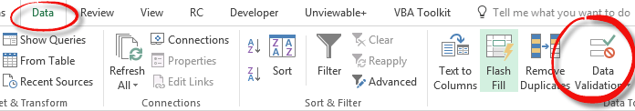
- Go to the Data tab in the ribbon.
- Click on Data Validation.
- In the dialog box, set the Allow box to List.
- Enter the values you want in the list, separated by commas, in the Source box, or select a range of cells containing the values.
- Click OK to create the drop-down list.
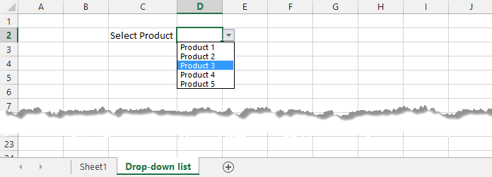
Step-by-step guide to insert a drop-down list in Excel
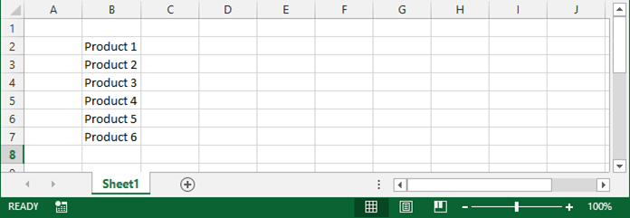
1. First, we have to create a sheet with all the names of our products for further calculations.
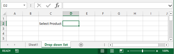
2: Create a new sheet, ’Drop-down list’, then create the drop-down menu in cell D2. Select a cell where you want to put the drop-down list (cell D2 in our example)
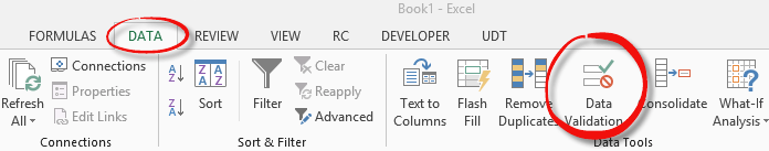
3: The Data Validation: Go to the ribbon and select the “Data” tab and click it. Click the icon “Data validation” on the ribbon.
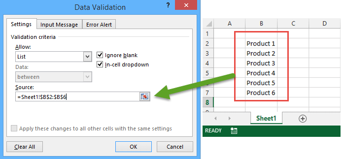
4: – In the pop-up window, we have to click the drop-down menu to select the data validation method we want to use. Okay, choose “List” from the menu.
There are more validation options: (Any value, Whole number, Decimal, Date, Time, Text length, and Custom)
In the Source field, add a range =Sheet1!$B$2:$B$6
Click OK.
This will create a drop-down list that lists all the product names.
What is the dependent drop-down list?
We might need a solution that the simple list cannot solve. For example, how can the list be a two-level dependent list?
This means that there are two drop-down menus, and the elements appear in the second one depending on the choices we made in the first one.
A little explanation:
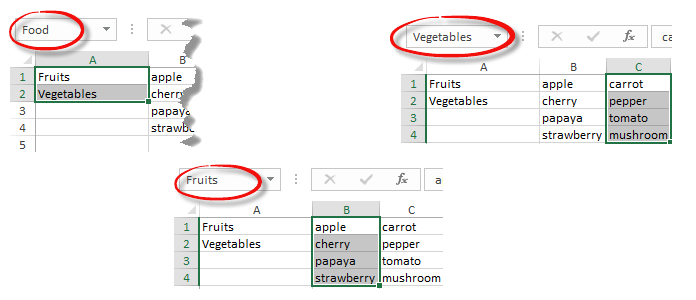
Just think of a simple example. We have 20 kinds of different vegetables and 20 different fruits. We want to classify all the elements into two categories. The first list contains two types: vegetables and fruit. Only those elements dependent on the first list will appear in the second list.
So when the first category is fruit, amongst the elements of the second list, we will not see, for example, the pepper, only the fruits. The vegetable category works the same way.
Finally, let’s see this method with the help of an example; we describe how to create dependent drop-down lists in Excel.
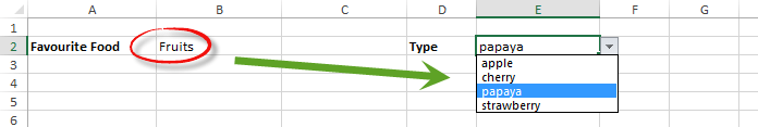
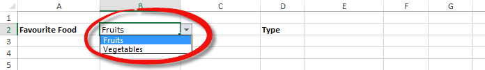
The user selects Fruits from a drop-down list.
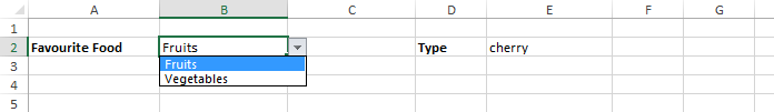
As a result, a second drop-down list contains the Fruits items.
1: On the second sheet, create the following named ranges. Select the range, type a name into the Name Box, and press enter.
2: On the first sheet, select cell C1.
3: Go to the Data tab on the ribbon; click Data Validation in the Data Tools group.
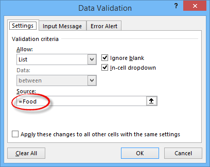
The ‘Data Validation’ dialog box appears.
In the Allow box, click List. Next, click in the Source box and type =Food.
4: Click OK and check the result.
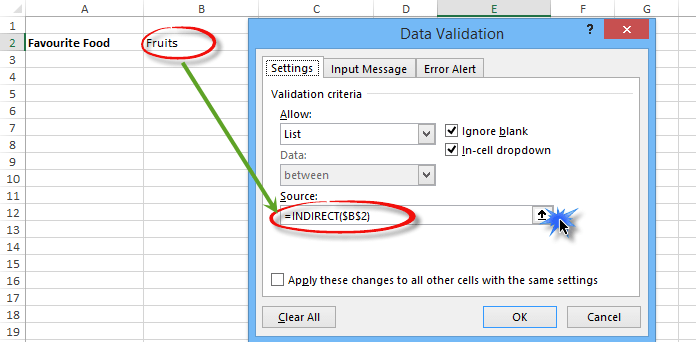
5: Next, select cell E2.
6: In the Allow box, click List.
7: Click the Source box and type =INDIRECT($B$2).
Click OK. See the results in the picture below!
Just a few words about the INDIRECT() function:
The INDIRECT function returns the reference specified by a text string. For example, the user selects Fruits from the first drop-down list. Therefore, =INDIRECT($B$1) returns the Fruits reference. As a result, the second drop-down list contains the Fruits items.
Conclusion
Let’s assess what we have learned today! First, more and more people get to know and use the possibilities of data validation. Of these, the most common is the drop-down regulation, when we prescribe the input or choices of a roll-down menu that can be entered into a chosen cell.
Do many people use the file, and everyone inputs the data differently? Only you can use it, but would you like to filter your own mistyping? Maybe you send the Excel table to partners, and you want to be sure they fill out the correct information. Data validation is the solution to all these cases. Download the sample workbook!