Learn how to find and get the last word from a text string using the MID, FIND, CHAR, LEN, and SUBSTITUTE functions.
Working with text strings in Excel is sometimes an easy task, sometimes not. In this article, we will explain how to use the best practices. As usual, first, we will perform the task using Excel’s built-in string manipulation functions. Furthermore, we’ll introduce the new user-defined function, GETLASTWORD to write better formulas faster.
How to extract the last word from a text string
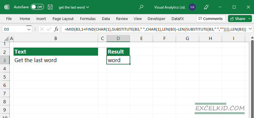
Steps to extract the last word from a text:
- Select cell D3.
- Type =MID(B3,1+FIND(CHAR(1),SUBSTITUTE(B3,” “,CHAR(1),LEN(B3)-LEN(SUBSTITUTE(B3,” “,””)))),LEN(B3))
- The formula extracts the last word between delimiters.
Explanation
- =LEN(B3)-LEN(SUBSTITUTE(B3,” “,””)): First, we’ll replace the space characters with empty strings.
- =SUBSTITUTE(B3,” “,CHAR(1),LEN(B3)-LEN(SUBSTITUTE(B3,” “,””))): After that, insert a delimiter CHAR(1) for the last space.
- =FIND(CHAR(1),SUBSTITUTE(B3,” “,CHAR(1),LEN(B3)-LEN(SUBSTITUTE(B3,” “,””)))): FIND the location of the delimiter in the selected string.
- FIND(CHAR(1),SUBSTITUTE(B3,” “,CHAR(1),LEN(B3)-LEN(SUBSTITUTE(B3,” “,””)))) + 1: Because we are using a delimiter, we have to strip the first character of the last word.
- =MID(B3,1+FIND(CHAR(1),SUBSTITUTE(B3,” “,CHAR(1),LEN(B3)-LEN(SUBSTITUTE(B3,” “,””)))),LEN(B3)): Finally, expand the formula with the MID function to extract the last word between the delimiter’s location.
Get the last word using TRIM and RIGHT functions
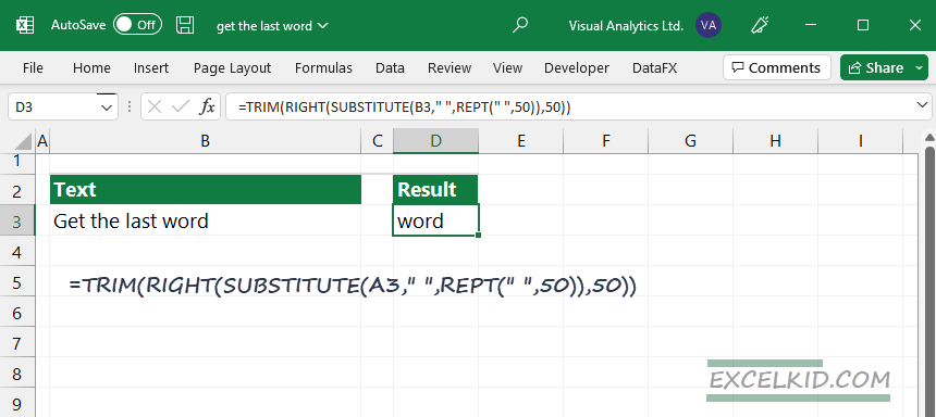
In the next example, we have the same goal. If you want to extract the last word from a text string, you can use another alternative calculation method: combine REPT, SUBSTITUTE, RIGHT, and TRIM. This method uses tricks and makes the formula mentioned above easier.
Let us analyze the following formula:
=TRIM(RIGHT(SUBSTITUTE(A3,” “,REPT(” “,50)),50))

The TRIM function will remove any number of leading spaces. We are using 50 as an argument, but in some cases (for example, you have long words), you need to increase this number. The SUBSTITUTE function finds all spaces in the text string and replaces each space with N spaces. N is an integer type variable, in this case, 50.
=SUBSTITUTE(A3,” “,REPT(” “,50))
The RIGHT function extracts N characters (50) from the right.
=RIGHT(SUBSTITUTE(A3,” “,REPT(” “,50)),50)
We have only one step left. The TRIM function removes extra spaces between words, leading, or trailing spaces. Finally, the formula returns the last word.
=TRIM(RIGHT(SUBSTITUTE(A3,” “,REPT(” “,50)),50))
Using GETLASTWORD function
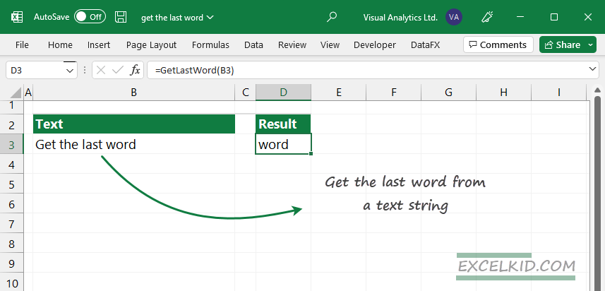
Last but not least, Speed matters. Of course, we have a user-defined function to boost your productivity. The syntax is easy to understand for everyone.
=GetLastWord(cell)
The function uses a single argument, “cell reference“.

We strongly recommend using a user-defined function library like DataFX. The add-in dramatically improves your productivity. Also, try the DataXL free Excel add-in for data cleansing projects. No coding skills are necessary; you must follow the add-in installation guide.
