
Subscript in Excel is a quick formatting option for decreasing text size or a number. Thus, the text is smaller after the operation. There are various methods for applying subscript: you can apply shortcuts and custom cell formatting, then use the subscript checkbox.
Properly formatting your data in Excel can make a huge difference in how easily it can be understood. One commonly used formatting technique is applying subscripts, which is particularly useful when dealing with scientific data, chemical formulas, or any text that requires certain characters to be presented in a smaller size below the normal text line.
This type of formatting is relatively straightforward, though it may not be as commonly known as other formatting options. This guide will walk you through the various methods for applying subscript formatting in Excel, helping you choose the one that best suits your workflow.
The shortcut is not short in this case, but much faster than other ways.
Ctrl + 1, Alt + B, Enter
How to use the Subscript Shortcut?
Steps to apply the subscript format in Excel:
- Select one or more characters you want to apply the subscript format.
- Use the Ctrl + 1 shortcut to open the Format Cells dialog box.
- Press Alt+B to mark the Subscript option checked.
- Press Enter to apply the shortcut.
If you are using Mac, apply these steps below:
- Click on the Formula bar and select the character you want to apply the superscript format
- Press Command + 1 to display the Format Cells dialog
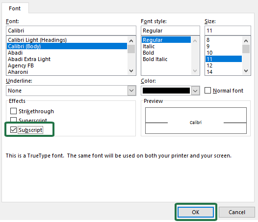
- Under the Effects Group, click the checkbox for subscript.
- Click OK.
Windows Shortcut
then
Mac Shortcut
then
use the subscript checkbox.
Excel Subscript Examples
While Excel offers built-in features for applying subscript formatting, there are times when you may need to use alternative methods. Beyond the traditional shortcut and format cell options, Excel provides more advanced methods, such as creating macros to apply subscript formatting to selected text quickly.
Add a Shortcut using a Macro
We always support the faster way to solve a problem. In the first example, we’ll show you how to use a short macro to apply the subscript shortcut effectively. These workarounds are especially useful if you frequently need to adjust formatting. One of the most powerful methods we’ll cover is using a simple VBA macro.
The macro will use a parameter – str – (you can add it using an input box) to calculate the given position for the format.
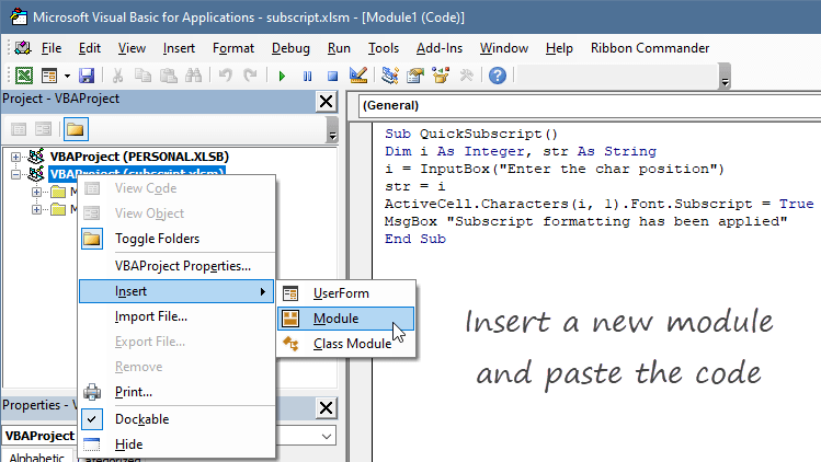
To insert the new code, follow the steps below:
- Press Alt + F11 to enter the VBE (Visual Basic Editor)
- Right-click on the Workbook and choose ‘Insert new module.’
- Paste the code, then save the Workbook to a macro-enabled format, like .xlsx or xlsb.
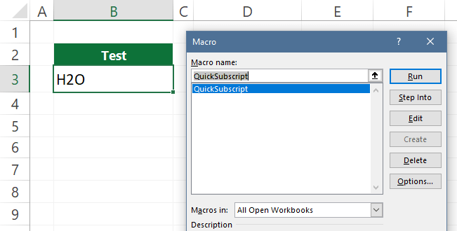
To run the macro, click on the Developer Tab and select macros. Pick our new macro from the list, then run it!
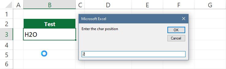
Enter a value (number) where you want to apply the subscript format.
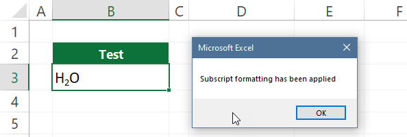
Click OK to apply the subscript on the selected cell.
Here is the code:
Sub QuickSubscript()
Dim i As Integer, str As String
i = InputBox("Enter the char position")
str = i
ActiveCell.Characters(i, 1).Font.Subscript = True
MsgBox "Subscript formatting has been applied"
End Sub
Cell Edit mode
The first method to apply a subscript in Excel is to switch Excel into the cell edit mode using the Edit cell shortcut, F2.
Here are the steps below:
- Double-click or press F2 to edit cell
- Select the character; Excel will highlight it
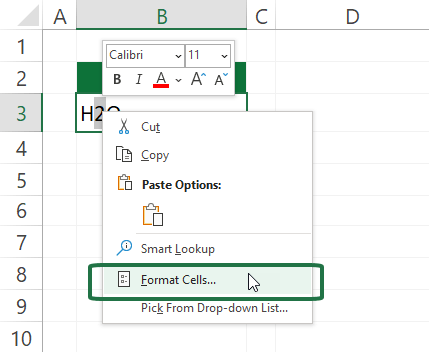
- Click on Format cells
4. The Format Cells dialog box appears
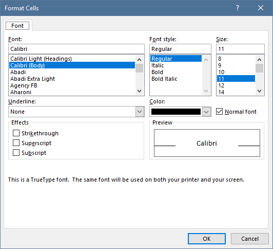
5. Select the checkbox under the Effects Group. Next, click OK.
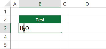
The result is the same as the previous example. Excel will apply the formatting on the second character of the text.
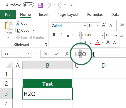
Apply Subscript formatting using the Formula Bar
You can apply the formatting by editing the text using the Formula Bar.
- Select the cell that contains text, then click on the Formula Bar.
- Select the character that you want to format.
- Right-click to open the Format Cells dialog box.
- Make sure the subscript checkbox is active.
- Close the dialog box by clicking OK.
Recommended articles
Thank you for reading our guide on how to use subscript in Excel. We recommend you use shortcuts for time-saving purposes. If you are interested, here is a list of our related articles:
- How to use the Fill Down Shortcut
- Shortcut to open the Insert Function Dialog Box
- Excel Cut Shortcut
- Superscript in Excel
- Strikethrough Shortcut