
Conditional formatting shapes and cells! This is an exciting area in Excel. This tutorial will show you how to use conditional formatted shapes using various techniques.
We will show you all the tricks related to this subject. You can create dynamic presentations using this Excel feature. We provide free downloadable spreadsheets and examples. Let’s start reading!
Formatting cells is a useful function. Can this function be extended? Is a shape fit to be the highlighted element of an Excel dashboard? Of course! Stay with us today, and we’ll show you how all this is possible.
Using Linked Pictures
It may appear that conditional Formatting in Excel only works with cells. But what if we would like to use formulas?
There’s no problem. Let’s use the simplest and most obvious solution. This is the linked picture method.
Let’s see step by step how to create it:
First, select an already formatted cell.
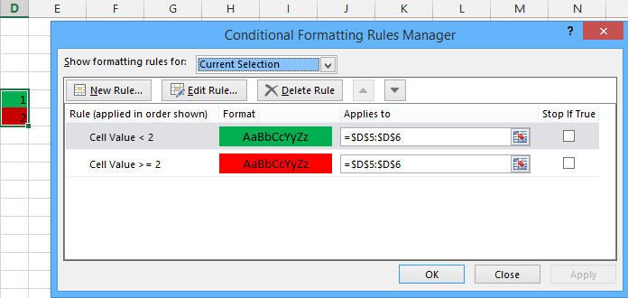
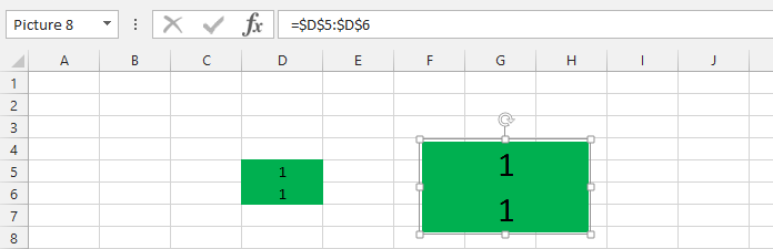
In the picture below, we have created a little example of this. We will pay attention to the range D5:D6.
You can see the rules in the Rules Manager window. We didn’t make it overly complicated. If the cell value is larger or equal to 2, it will color red.
If the cell value is smaller than 2, it will color green.
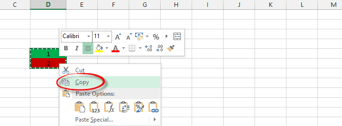
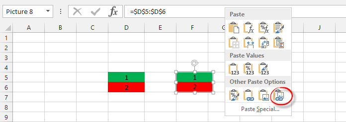
Copy the cells containing the conditional Formatting as a linked picture.
We can use the Home tab on the ribbon, but it is easier to use the right-click menu.
The linked picture acts as a graphical object. So, for example, we can move or resize it.
Enter 1 in both cells.
As an effect of the conditional Formatting, both cells will turn green, so the rule we have set will prevail.
We can control the shape with the change in the cell’s value.
This was, in any case, the simplest solution for using Conditional Formatting on a shape.
Don’t forget that now we are talking about a simple picture.
Can Conditional Formatting control shapes?
The answer is yes! And with an easy way. Some people like to overcomplicate VBA programming. There’s no need for that.
Following the tutorial furthermore, we’ll introduce two more methods.
Now we’d like to color a real Shape with the help of conditional Formatting. The first thing that comes to mind is to write a short VBA code.
The colors of the shapes are very easily controlled with the help of Visual Basic.
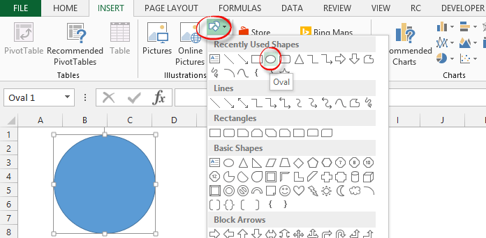
Insert a simple object.
We want the object’s color to change based on the cell’s value.
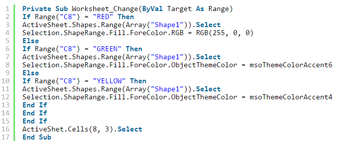
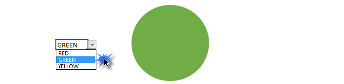
If the cell contains the word “RED,” the VBA code will color the circle red. The same principle will also be true for the “YELLOW” and “GREEN” variants. We start from the desire that we don’t want manually run any code or assign it to buttons.
Instead, start the code with the event of Private Sub Worksheet_Change (ByVal Target As Range).
This event ensures that a little VBA program will run if anything changes on the worksheet.
The explanation for the VBA codes:
If the value of the C8 cell = “RED” will highlight the shape Shape1 found on the active worksheet, it changes its color to red. In other cases (for example, if the C8 cell doesn’t contain the word “RED”), it will do the following.
If the text is = “YELLOW,” it will color the object yellow.
And if the C8 cell contains the word “GREEN”, it will color it green.
We are done with this.
It’s not very hard to create this code.
We don’t need at all advanced knowledge of VBA.
In a matter of moments, we can find the name and the changed color code with a macro recording.
Apply an Automated VBA Solution
Finally, we introduce a solution we recommend to everyone who is creating an Excel dashboard using conditional Formatting. VBA development is not always a grateful thing, but it’s time to announce the good news proudly. This macro is little but a very well-applicable solution.
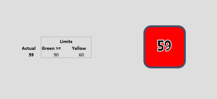
This small Excel file finally bridges over Excel’s sometimes extremely frustrating limitations. With the help of the conditional formatting shapes method, we again will push the limits of Excel. We’ll show the result before we get into the middle of it.
As you can see in the picture above, the shape’s color depends on the given value in the cell. Therefore, it will change dynamically depending on the size of the values. Now, in brief, we demonstrate how to use the template:
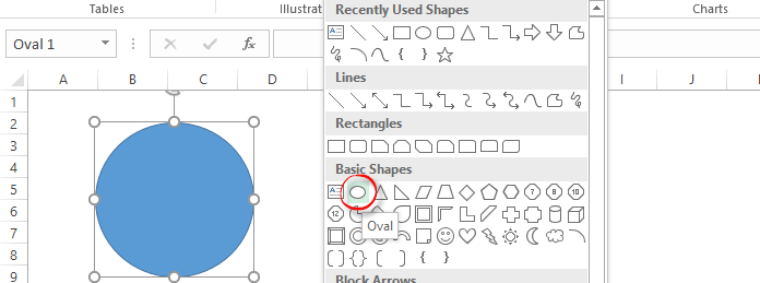
1. Insert a shape on any given worksheet.
2. We choose the oval object:
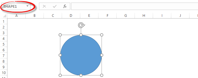
3. In the Name Box, change the default name to any given name:
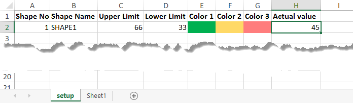
Why is this important? We store the values and colors that make the object dynamic on the setup sheet. We give every object a specific name and can easily identify them.
4. Let’s take a look at the setup worksheet!
The meaning of the columns:
Column A: This is an ID, don’t carry any importance; we can write anything here.
Column B: the name of the object. This must be the same one we wrote in the Name Box a minute ago.
The Upper Limit is the number above which the shape’s color turns green (Color1).
The Lower Limit is the number below which the shape turns red (Color3).
Between the upper and lower limits, the shape’s color will be yellow (Color2).
5. The colors can be arbitrarily changed.
6. Actual Value: doesn’t need any explanation. It is the current value.
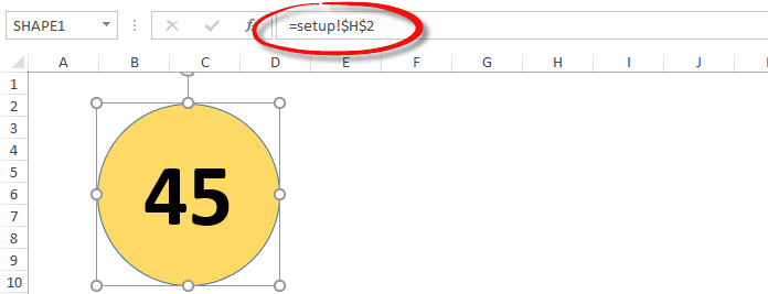
7. Let’s go back to Sheet 1.
Highlight the object, and in the Formula Bar field, type in the following:
=setup!$H$2This will set the current value to 45. Then, based on the table, the shape will change its color to yellow because this value is between the upper and the lower value range.
We can freely insert newer rows, and you can automatically command more shapes anytime.
You can create great-looking widgets and variance charts in minutes!
Conditional Formatting shapes: Improve your Excel skills
In conclusion, conditional formatting shapes can do more things than most think. You can find the VBA code in the sample workbook, which you can use and modify.
There are many possibilities in Excel. We’ll try to introduce as many of them as possible. See you next week! The macro-enabled worksheet can be downloaded from here!