
Learn how to remove duplicates in Excel using quick and creative methods. Finding unique values or removing duplicates is helpful when working with large data tables.
We will show you how to use Excel’s built-in data cleansing tools to find unique values in single or multiple columns.
Here we go; let us see how it works.
Table of contents:
- How to remove duplicates in Excel for a single column
- Find and remove duplicates for multiple columns
- Filtering for unique values and removing duplicate values
- Find and remove duplicate values using Conditional Formatting
- Remove duplicate data using Power Query
- Use the Excel UNIQUE function to remove duplicates
- Working with Pivot Tables
- Find and remove duplicates using Formulas
- Build a macro to remove duplicate values
- Use DataXL free add-in
What is a duplicate value? Things to consider…
A comparison of duplicate values depends on what appears in the cell. So, it’s not about the original value stored in the cell. Check the example below!
Our range contains the same date value in multiple cells with various formatting. If we apply the ‘Remove duplicates’ command, we will get unique values without duplicates. Why? We are talking about unique values, but the cell format is different!
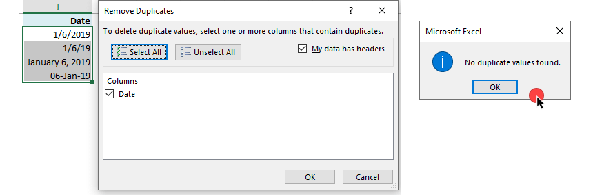
We recommend formatting the data before you start using the function. The remove duplicates tool will permanently delete your duplicates.
How to remove duplicates in Excel for a single column
In the first example, we’ll show you how to check for duplicates from a single column (list) and keep unique rows. First, select the range that contains duplicated values.
1. Locate the ribbon and click on the Data Tab.

2. A new window will appear when clicking on ‘Remove Duplicates.’
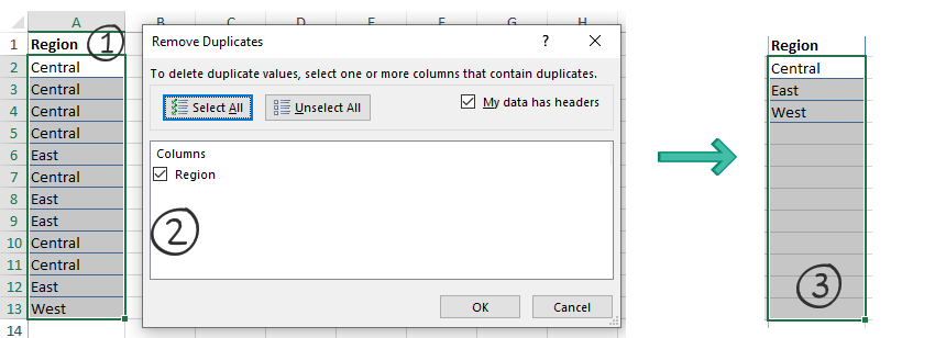
3. Finally, click the OK button. A small message box will appear. It contains helpful information about the number of removed duplicates and unique values. Click OK to close the window.
Important: Now, decide whether your data contains a header. If your range has a header, ensure the status of the ‘My list has headers’ box is checked. Otherwise, you’ll get a false result.
Find and remove duplicates for multiple columns
If you want to remove duplicates in multiple columns (and keep unique rows), use the following method. At first glance, the’ Remove Duplicates’ tool in Excel seems like a Swiss knife. But we kindly ask you to use it carefully. We’ll show you why. The results can differ when using the tool on a range containing multiple columns.
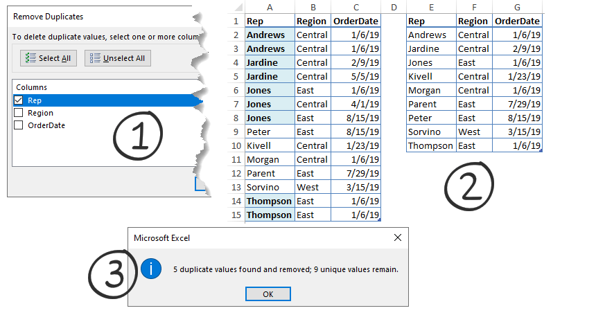
The examples below include three sample outputs for the ‘Rep,’ ‘Regions,’ and ‘OrderDate’ columns. First, as we mentioned before, click on the ribbon and select the ‘Remove Duplicates’ command.
Example 1
The first image displays all the duplicates based only on the Sales rep. After removing duplicates, nine unique values remain.
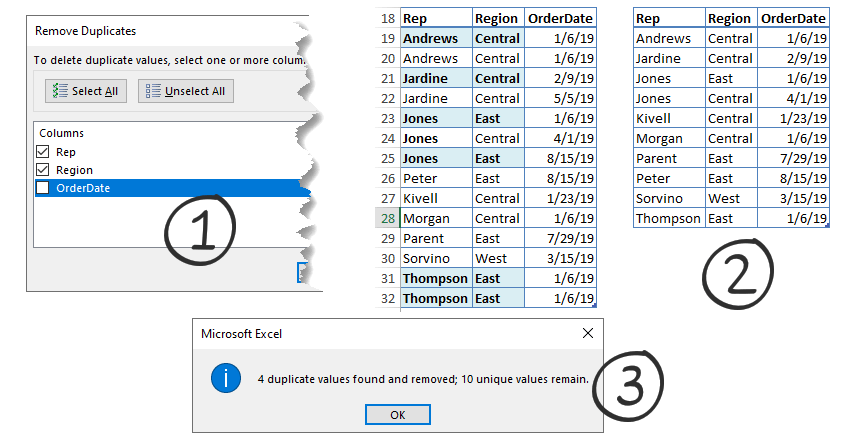
Example 2
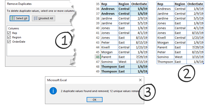
The second image shows all the duplicates based on the Rep and Region columns. After clicking OK, Excel removes four duplicate values based on two columns, leaving ten unique values.
Example 3
The third image shows all the duplicates based on all columns in the table. In this case, 12 unique values remain.
Remember: Before we start, let’s quickly compare removed items to check how the different filters work. Depending on your task, you can check for duplicates differently.
Filtering for unique values and removing duplicate values
This part of the tutorial will explain the differences between filtering (hiding) and removing duplicate values. At first glance, there are two similar tasks: their objective is to create a list of unique values.
Applying filters before removing duplicates is a smart decision. To avoid unexpected results, try switching the advanced filter on or using simple conditional formatting.
To filter unique values, follow the steps below.
1. Select the range or a table. Tip: Selecting a single cell in a range is good enough.
2. Click the Data Tab and select the ‘Advanced Filter‘ under the ‘Sort & Filter’ group.

3. Now, the ‘Advanced Filter’ box appears. You have two choices when applying the filter.
In the first example, we temporarily hide the duplicate values and keep the list in place. To do that, select ‘Filter the list, in-place,’ and check the ‘Unique records only’ box. Then, click OK to close the window.
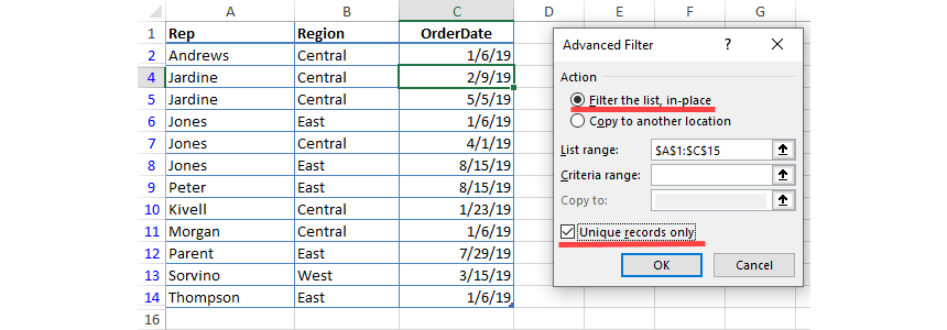
Check the result! If you use an advanced filter for unique values, duplicates are only temporarily hidden. Take a closer look at the picture below! This is a filtered list that contains all records.
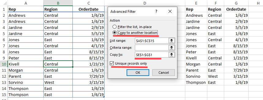
In the second example, we’ll show you how to copy the unique records to another location and keep the original list in place. To do that, select the ‘Copy to another location’ checkbox, then select the unique records only. Click OK. Finally, select the target location to copy the result to another worksheet.
Find and remove duplicate values using Conditional Formatting
Conditional formatting is a versatile tool; we love it! Let’s see how to highlight duplicate values in a single column:
- First, we have to talk about an important step. It’s important to select all cells in a range! It is a limitation of formatting rules.
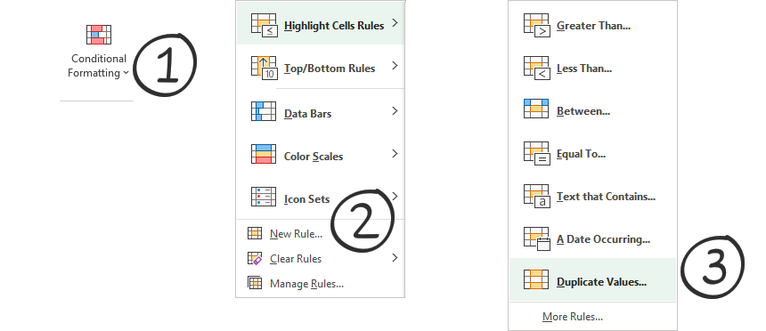
- Go to the Home tab and locate the Style group.
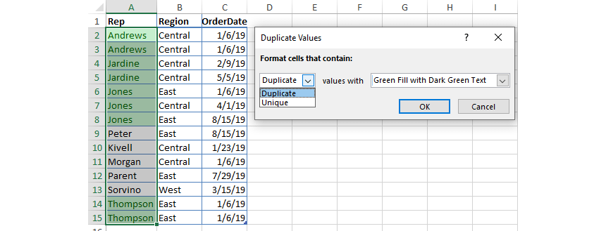
- Click the small arrow for Conditional Formatting from the drop-down list, then click Highlight Cells Rules. Finally, select Duplicate Values.
The method is perfect for removing duplicates in a single column.
How do you find unique or duplicate values using multiple columns? We will apply a small trick because conditional formatting cannot work with records across rows. First, create a helper column and use the CONCAT function to create a single string without spaces.
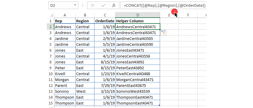
We’ll use this combined column to check for duplicates in more than one column.
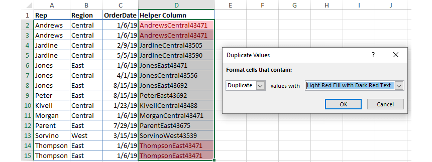
The first three steps are the same as the single-column example:
Click Conditional Formatting > Highlight Cells Rules > Duplicate values. Select the’ Duplicate’ option from the drop-down list to highlight the duplicate values for three columns. Then, apply a built-in or a custom formatting style. The result is below:
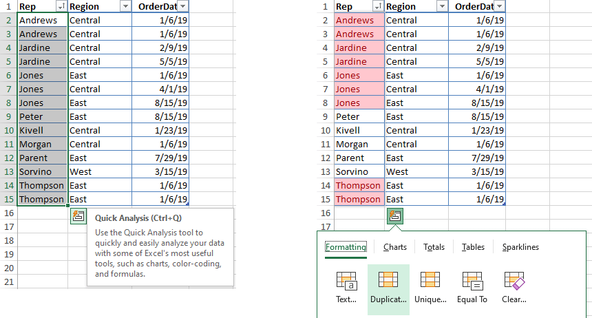
Tip: If you need a quick overview of duplicates, use the Quick Analysis Tool.
Select the range that contains duplicates. A small icon will appear at the end of the range. Choose the ‘Formatting’ tab and select ‘Duplicates’ from the list. You can use the ‘Ctrl + ‘Q’ shortcut too.
Find And Remove Duplicate Data using Power Query
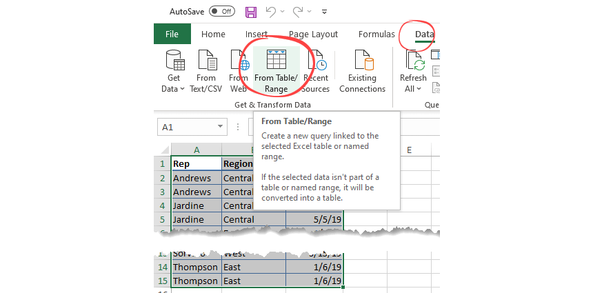
Select the range you want to add to the Power Query Editor. Then, select the Data Tab in the ‘Get and Transform’ section and choose the ‘From Table / Range’ option.
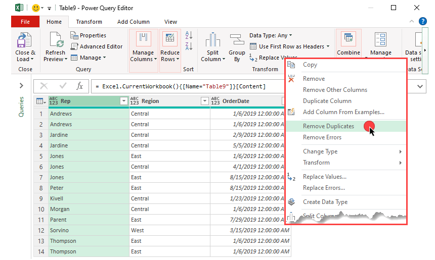
The Power Query window now appears. In this case, select the first column, ‘Rep.’ Right-click and apply the ‘Remove Duplicates’ command.
Working with multiple columns
The Power Query-based method works on single or multiple ranges.
Example 1: If you need to find duplicate rows based on the entire table, hold the ‘Control’ key and select the column by clicking headers.
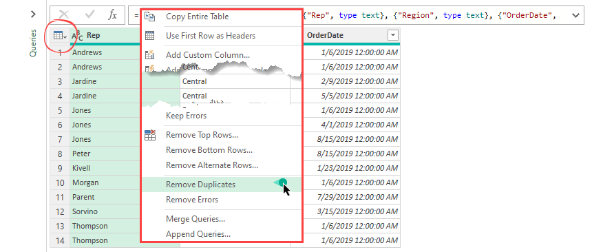
Example 2: Quick tip to keep distinct values based on the entire range: Check the table icon on the first column’s header. Right-click, then click Remove duplicates. It’s easy!
Pivot Tables
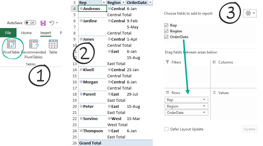
In this example, we’ll show you how to remove duplicates using Pivot Tables.
- Select data.
- Click the Home Tab and Insert a Pivot Table.
- Make sure to drag all three fields into the Rows section.
Go to the Design Tab and transform the Pivot table using the steps below.
Click on the Pivot Table area:
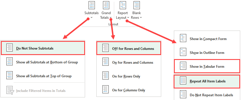
- Select ‘Subtotals’, and click ‘Do Not Show Subtotals‘
- Switch off showing ‘Grand Totals’ using the drop-down list
- Under the ‘Report Layout’ section, click ‘Show data in Tabular Form’ and ‘Repeat All Item Labels’
It is good to know that the Pivot table lists only unique values. If you create a proper report layout, the Pivot table removes duplicate rows.
Find and remove duplicates using Formulas
A comparison of duplicate values depends on what appears in the cell. So, it’s worth using formulas and functions to remove duplicates properly.
Let’s see the example: We will create a helper column and join the data in three columns. But first, add a name to the new column, in this case, ‘Joined records.‘
Combine the records using the Excel CONCAT function:
=CONCAT(Rep, Region, OrderDate)
With the help of the COUNTIFS function, we’ll take a quick overview of the number of duplicate values. Create a new column, ‘Count Duplicates.’ Enter the formula, then evaluate:
=COUNTIFS($D$2:$D$15,D2)
The result:
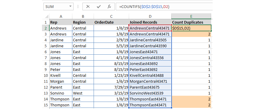
Copy the formula down until cell E15. The COUNTIFS function will show the duplicates quickly.
Take a closer look at the output:
- We are talking about distinct values if the result = 1
- If it’s greater than 1, the value appears in the list more than once
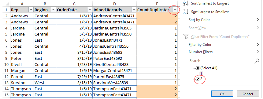
I’ve just highlighted the duplicate values using orange fill. To remove duplicates, apply a filter using the Ctrl + Shift + L keyboard shortcut and select the duplicate rows using the drop-down list.
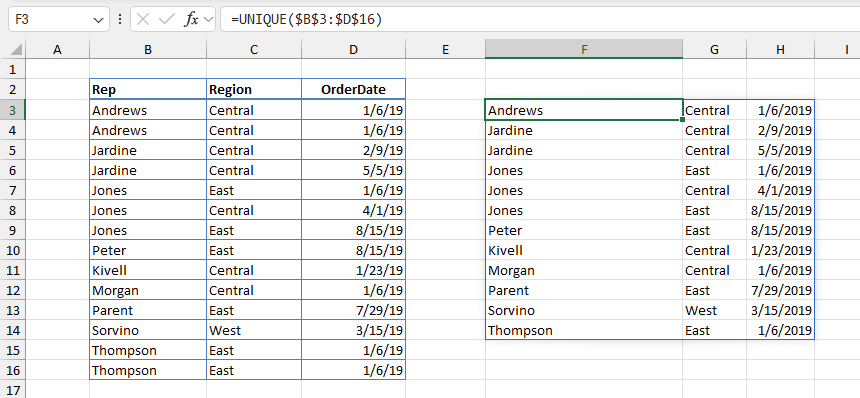
Using the UNIQUE function
The UNIQUE function allows you to create a unique list in one step. This function is currently available only to Microsoft 365 subscribers.
Use a macro to remove duplicate values
If VBA is your friend, we’ll show some small snippets to keep unique rows.
- If the range does not have a header, then use Header:=‘xlNo’
- If the range has a header, then use Header:=‘xlYes’
Example 1: Our range is A1:C15, which has a header, and we want to remove duplicates from the first column. The code is the following:
Sub Example1()
Range("A1:C15").RemoveDuplicates Columns:=1, Header:=xlYes
End Sub
Example 2: The range is the same as above, and we want to remove duplicates from the first and the third columns:
Sub Example2()
Range("A1:C13").RemoveDuplicates Columns:=Array(1, 3), Header:=xlYes
End Sub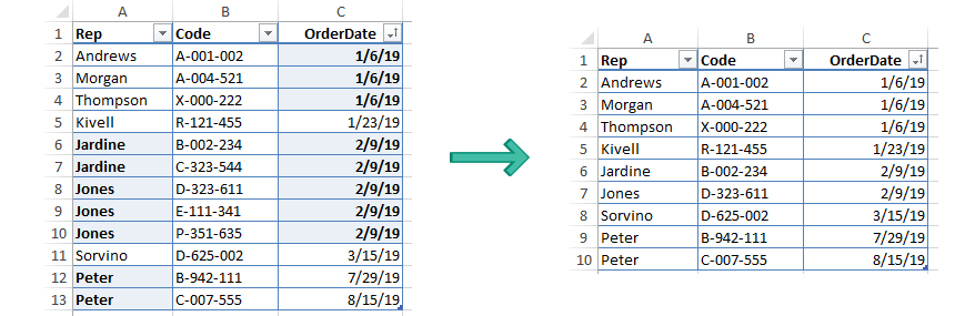
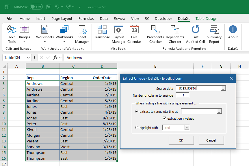
Use DataXL free add-in
DataXL is our answer to data cleansing challenges! This small add-in dramatically improves productivity.
Additional resources: