Learn how to create a dynamic HR KPI Dashboard Template in Excel using grid layout, multiple KPIs, and advanced chart types.
This tutorial will show you how to build a Human resource template from the ground up. To make the template dynamic, we’ll use custom charts, infographics, and a drop-down list.
Create a Human Resource KPI Dashboard
Before we discuss the details, you can download the practice files. You’ll receive two spreadsheets, the light and the dark versions.
Prepare Data
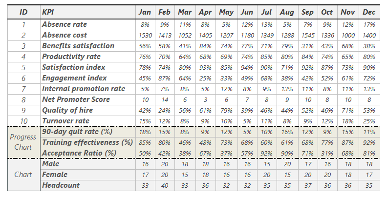
We’ll use the following data set as an example. The first ten rows show various key performance indicators, from the Absence rate to the Turnover rate.
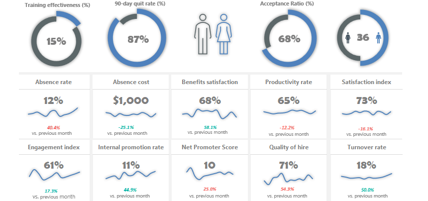
We use progress charts to visualize four highlighted indicators:
- 90-day Quit Rate (%)
- Training Effectiveness (%)
- Acceptance Ratio (%)
- Head Count (%)
We follow the common dashboard design rules, so our initial data set is in the ‘Data’ Worksheet, and we perform calculations and insert a new Worksheet, ‘Calculations’. Here, let us calculate the variance between the selected month and the last month. Furthermore, to make our dashboard dynamic, we link the drop-down list results from the Dashboard sheet to the ‘Calculations’ sheet.
Use the following formula to get the value based on the drop-down list selection.
Type in cell V6:
=IF($F$5=$T$4,F6,IF($G$5=$T$4,G6,IF($H$5=$T$4,H6,IF($I$5=$T$4,I6,IF($J$5=$T$4,J6,IF($K$5=$T$4,K6,IF($L$5=$T$4,L6,IF($M$5=$T$4,M6,IF($N$5=$T$4,N6,IF($O$5=$T$4,O6,IF($P$5=$T$4,P6,Q6)))))))))))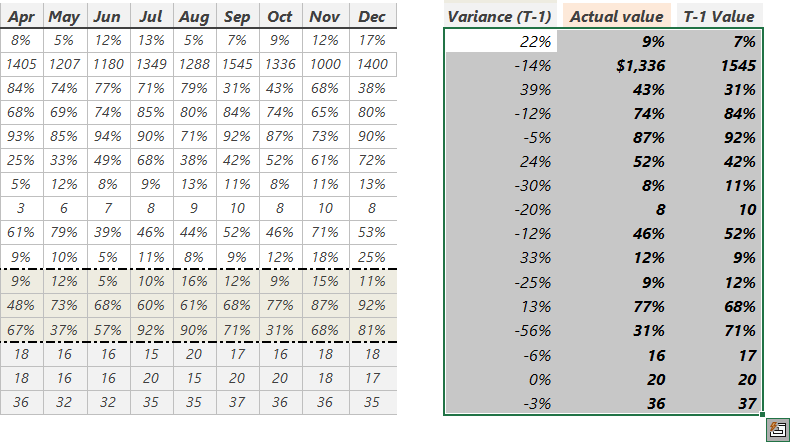
Use the formula in cell X6 to get the T-1 value:
=(IF($T$4=$F$5,F6, IF($T$4=$G$5,F6, IF($T$4=$H$5,G6, IF($T$4=$I$5, H6,IF($T$4=$J$5, I6, IF($T$4=$K$5, J6,IF($T$4=$L$5,K6,IF($T$4=$M$5,L6,IF($T$4=$N$5,M6,IF($T$4=$O$5,N6,IF($T$4=$P$5,O6,IF($T$4=$Q$5,P6,"")))))))))))))Finally, get the Month-by-Month result:
=(V6/X6)-100%Insert a Drop-down list
If you want to create a KPI scorecard, use a drop-down list. This small form of control helps us select the month we want to display. For example, as mentioned earlier, we use 12 months to track and analyze the KPIs.
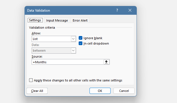
Click the Data Tab on the ribbon, select Data Validation, then choose the Data validation command. Under the validation criteria tab, choose the ‘List’ option. Under the ‘Source” Group, browse cells containing the month’s names.
Create a Card layout
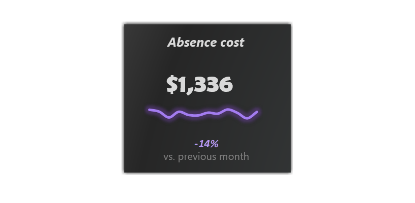
Take a closer look at the data visualization. In this case, you can find useful information. Using a panel chart style, our HR KPI template displays the indicator’s name, actual value, and trends. We also need to show the variance between the actual and previous months.
Steps to create a card:
First, add a data label for the card. Insert a text box, type an equal sign, and connect the KPI name from the ‘Data’ worksheet. The label is dynamic since we have a link between the data and the ‘Dashboard’ worksheets.
Next, select the monthly data on the ‘Data’ sheet and insert a line chart. The next step is to add the actual value to the card. Select the cell in which the link contains the actual value and link it to the ‘Dashboard’ Worksheet. In the last step, we will display the variance between the selected and the previous month’s data. Use the ‘Calculation’ Worksheet to link the data to the card.
Conditional formatting is a must-have tool if you want to highlight cells. So, if you find a space-saving solution, use scorecards to present your data.
Metrics
It is important to pick the proper key performance indicators. As usual, the dashboard has limited space, so focus on the relevant metrics. Key Performance indicators play an important role, and we will show the frequently used HR metrics:
- Training effectiveness can help us determine what parts of the training works well and what parts need to improve.
- The acceptance Ratio is 80% if ten candidates and eight candidates accept job offers in the period.
- 90-day quit rate uses the formula: (terminated contracts / new hires) * 100
- Absence Rate: the number of absence days as a percentage of workdays.
- Absence Cost is the cost of an employee’s habitual absence from work.
- Benefits satisfaction is the level of contentment employees feel with their job.
- Productivity rate: It’s simply: Output / Hours worked
- Satisfaction index: gives us feedback on how satisfied employees are with their current situation.
- The engagement index results from a survey in which employees assess their engagement at work.
- Internal promotion rate evaluates the rate at which open positions are filled using an internal promotion within the organization.
- Net Promoter Score: We are using it with a single-question survey.
- Quality of hire shows how much a new hire contributes to a company’s success.
- The turnover rate is the % of employees left a company within a given period.
Additional resources: