Learn how to use the percentile rank formula to classify data based on criteria.
We use percentile ranks often in data analysis. Using this feature, we can check the target performance of the group as a whole.
Highlight Data Based on Percentile rank
The problem
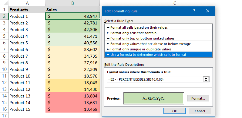
We have a list of 20 products with different sales. So instead of the top n% and bottom n%, we want to classify the products based on sales.
The solution
We’ll use a custom conditional formatting formula that contains the formulas based on the PERCENTILE function. Using the function is not rocket science; we must add only two arguments: the range containing data and the percentile score.
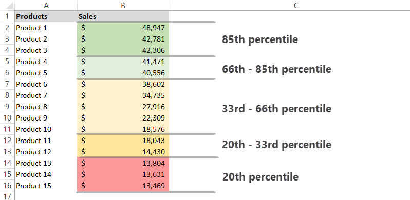
In the example shown, we split the range into 5 parts based on requirements. Next, we’ll use the following rules to apply different colors.
=B2>=PERCENTILE($B$2:$B$16,0.85) 'Highlight the top 15%
=AND(B2<PERCENTILE($B$2:$B$16,0.85),B2>PERCENTILE($B$2:$B$16,0.66)) 'Between 66% and 85%
=AND(B2<PERCENTILE($B$2:$B$16,0.66),B2>PERCENTILE($B$2:$B$16,0.33)) 'Between 33% and 66%
=AND(B2<PERCENTILE($B$2:$B$16,0.33),B2>PERCENTILE($B$2:$B$16,0.20)) 'Between 20% and 33%
=B2<=PERCENTILE($B$2:$B$16,0.2) 'to highlight the bottom 20% value
It is worth using the AND function if we want to find a range between X and Y.
Steps to create a classification
- Select the range which contains data. (in the example, range B2:B16). Click the Home tab. Select Conditional Formatting and New Rule. A dialog box will appear.

2. Locate the “Use a Formula to Determine Which Cells to Format” option. All applied formulas will be evaluated based on the rule. If the result is TRUE, the selected formatting style will highlight the range.
3. Now, enter the formula. In the example, we’ll find the top15% values in a range.
=B2>=PERCENTILE($B$2:$B$16,0.85)4. Click the Format button. The Format Cells dialog box will appear. You can customize the formatting style. Click OK, and we’ll return to the ‘New Formatting Rule dialog box’.
5. Click OK to validate the entered formatting rule.
6. At this point, you should be in the Conditional Formatting Rules Manager dialog box.
Repeat these steps to apply another four rules.

Tip: If you need to change your scenario, select a single cell in a highlighted range. Click on the Home tab and select conditional formatting. Select the Rules Manager dialog box. Choose the rule you want to modify. Click the Edit rule button.