
This article explains how to sort by cell color in Excel using conditional formatting, filter function, or VBA automation.
How to sort by cell color in Excel
Steps to sort by color in Excel:
- Select a cell inside the range that you want to sort.
- Use the Ctrl + Shift + L shortcut to turn the Filter on.
- A small arrow will appear in the header.
- Click the arrow.
- Choose the Filter by Cell color option and select the preferred color.
- Now you have a sorted list.

#1: Use the custom sort
1. Select your data range, which contains three columns. If you prefer using the shortcuts instead of the mouse, select the top-left corner of the data range and press CTRL+A.
2. Click the Data Tab on the ribbon. Click the Sort button.
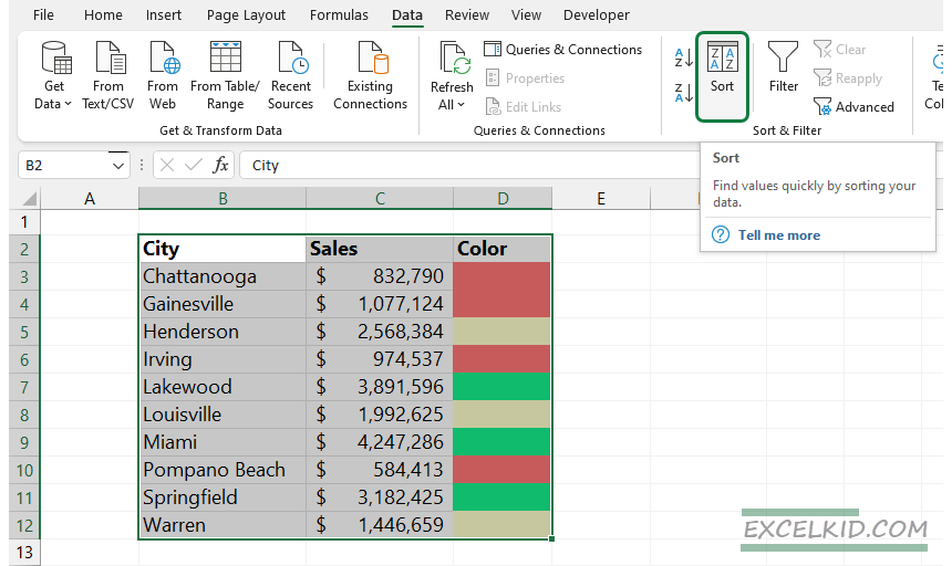
3. The Sort dialog box will appear.
4. Your data has headers; check it on the top-right corner of the dialogue box.
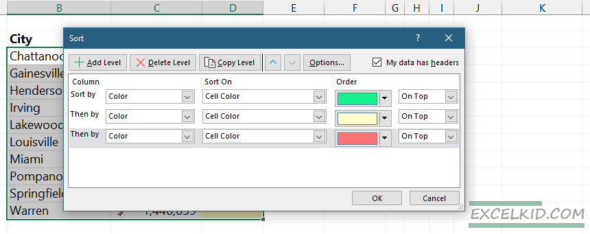
5. In the Sort by row, select Color.
6. Navigate to the Sort On label and select the Cell Color option from the drop-down list.
7. Select green as the fill color and set the Order value to On Top.
8. To add a new row, click the Add Level button.
9. Repeat the last step twice for the yellow and red fill colors.
10. Click OK to sort by color
Result:

#2: Sort by color using filters
You can use filters instead of sorting. We’ll show you how to filter the data if you want to learn a faster method.
1. Select the column that contains colors.
2. Under the Data Tab, locate the Sort & Filter group, then click the Filter button.
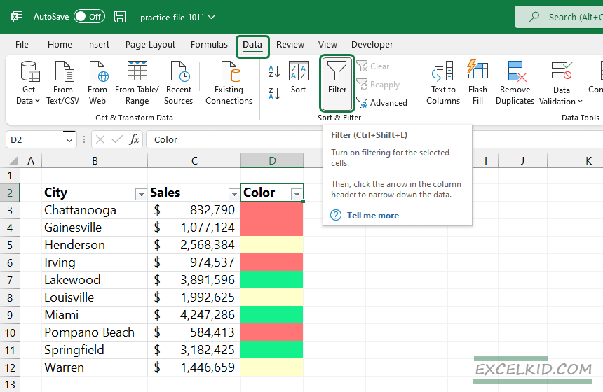
3. A small arrow will appear; you can find it in the header.
4. Click the arrow.
5. A new window will appear. Choose the Filter by color option and select your preferred color.
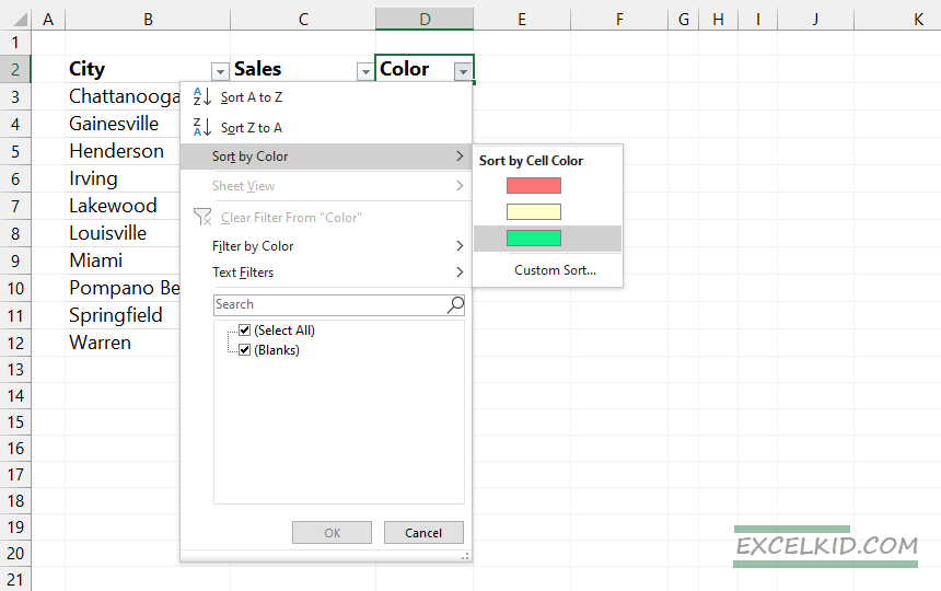
The function will sort the list by cell color.
#3: Sort a Conditionally Formatted Range based on colors (value-based)
If you have a list with conditional formatting icons (in this example, flags), you apply the classic scheme: the higher third values are green, and the lower third is red. Then, use the typical value-based sorting.
1. Right-click on the icon range.
2. Choose ‘Sort’, then click ‘Sort to largest to smallest’ option.
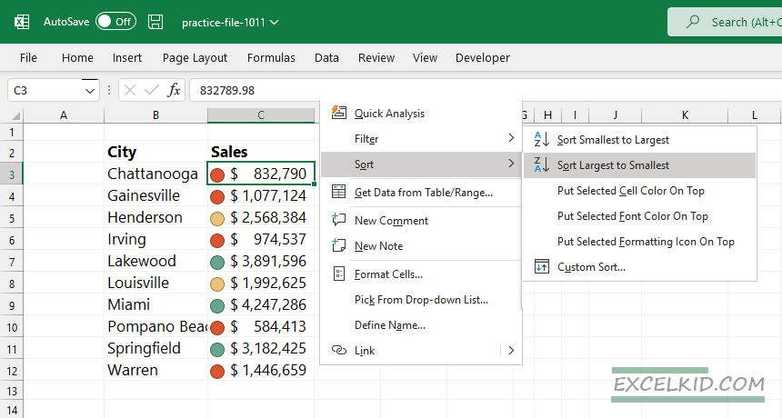
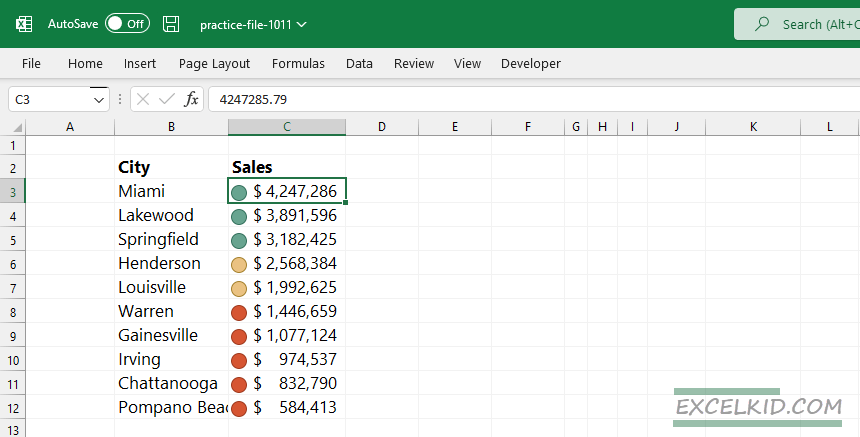
3. That’s all! You’ll get the same result as shown below.
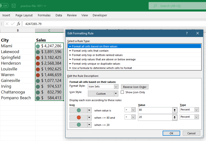
#4: Using Conditional Formatting Rules
Let us assume that your list was formatted based on a custom rule. You want to highlight the top 20% and the bottom 20% of the range using green to find the peaks (highest and lowest values in the array). In the next example, we want to sort data by color but cannot apply value-based sorting.
1. Select the entire data set, in this case, ‘C3:C12’. Right-click in the range and choose the Sort, Custom Sort option from the menu.
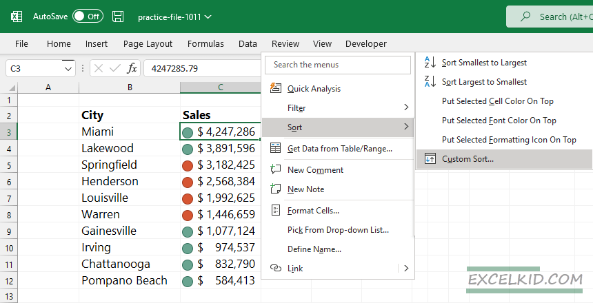
2. A new window will appear. First, select the column that contains colors.
3. Choose the ‘Conditional Formatting’ icon.
4. Select your preferred color in the Order section.
5. Finally, apply the ‘On Top’ parameter for proper sorting.
Click OK, and you will get a sorted list based on the selected color.
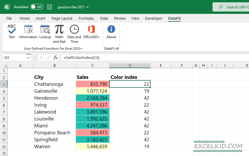
#5: Using User-Defined Function
- Install the DataFX add-in that contains a custom function library
- Enter the formula: =DxCellColorIndex(cell)
- As a result of the formula, you’ll get unique numbers, so from now on, it’s super easy to apply a custom sort based on values.
#6: Sorting rows by color using DataXL add-in
We love add-ins; with their help, we can boost productivity.
First, install DataXL Productivity Add-in. Select the data range, which contains values and colors. Go to the DataXL tab on the ribbon and choose Ranges. From the drop-down list, select the color-based sorting option.
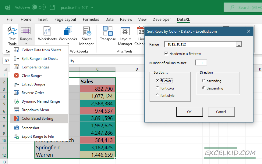
3. Now, you can sort data by fill color, font color, or font style. Check the “Headers in a first-row” checkbox if your range has a header. Then, click OK to apply a quick sort.