
The Excel Table is a relatively seldom-used and underrated feature in Excel. But in today’s article, we’ll show you its advantages. It makes it easy for users to manage data in a tabular format.
Converting a data range into a table makes its usage even easier. After this little intro, let’s see the step-by-step tutorial!
Convert tabular format into Excel Table
Suppose our data is in tabular format. In the next few steps, we’ll show you how to convert them into an Excel Table.
1. Select the worksheet range that contains the data set.
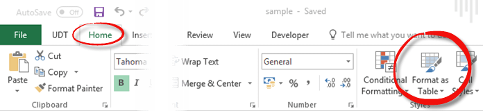
2. After this, choose the Home tab, then go to the Format as Table icon.
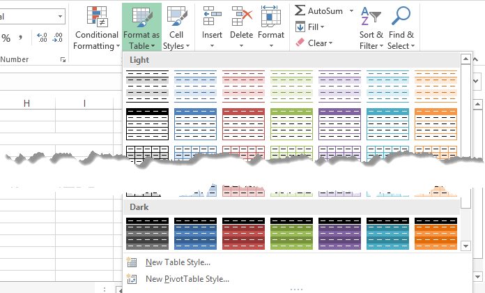
3. As you can see in the picture, many pre-set arrangements and color themes are available. Choose the one you like!
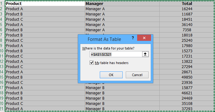
4. The Format as Table dialogue box contains the following information. First, “Where is the data for your table?”
The answer is obvious; we can see the range we want to convert into Table format. We always check this before the conversion to ensure the right range!
If our data table has headers, we must check the box “My Table has headers.” Excel will automatically insert headers into the first row if your data doesn’t have headers.
5. Click OK.
Shortcut tips: Use the Ctrl+T keyboard shortcut; this makes the conversion much faster. If you highlight the data table as an effect of the shortcut, you will immediately see the “Format as Table” dialogue box; there is no need to look for it on the ribbon.
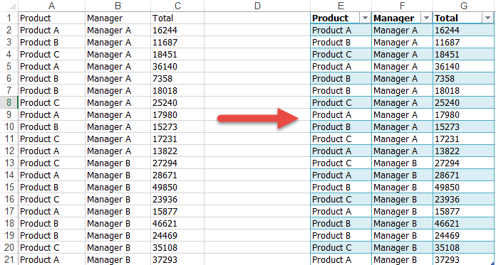
When your tabular data is converted into an Excel Table, your data will look as shown below.
The most important changes are that the header is darker and the rows’ colors are different. Data filters are enabled on the header. Note that the data hasn’t changed, only the design.
How do we convert data from the table into a tabular format?
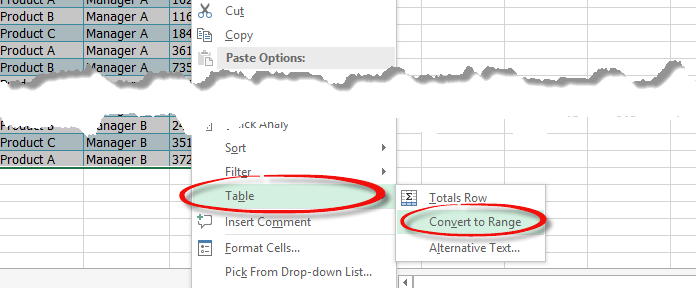
Sometimes, we want to convert the Excel Table to its original tabular range format. Let’s see what we have to do! Highlight the range or make it easier to click anywhere on the table. Right-click the “Convert to Range” icon from the Table menu.
Note that when you convert the Excel Table to a range, it no longer has the properties of an Excel Table (discussed below); however, it retains the formatting.
Useful Table Features in Excel
So we have seen how to create a table. Now let’s see the useful functions it enables.
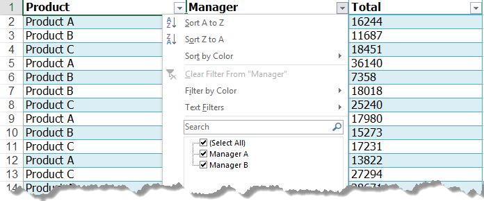
• The created table automatically creates a header enabling the sort and filter options.
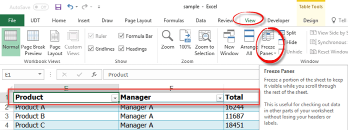
• If our list or range is long and stretches beyond the visible screen, the header remains at the top when scrolling. It works similarly to the “Freeze Top Row” function.
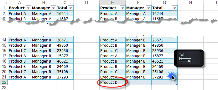
• And now let’s see one of our favorite functions! When we reach the bottom of our range but want to add additional rows, use the TAB button. This adds new rows to the table.
• Now, let’s examine the case when we need to do calculations with the table. When new rows are added, Excel automatically figures them into the calculation.
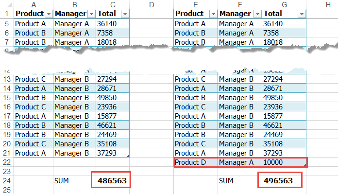
Table Design – Overview
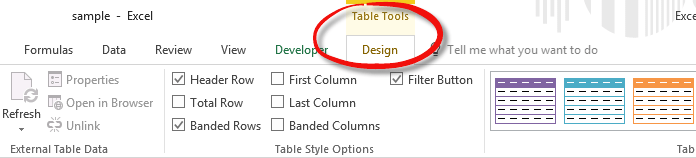
If you are involved with Excel, you know it is easy to customize. We can dress it any way we want to. Click on any cell in the Table, and an additional button, “Table Tools Design” will appear on the ribbon. This is optional and can be seen only when working with tables.
When you click on the Design tab, several options are available.
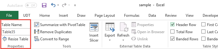
- Properties: Properties are one of the group’s most useful tools. We can give our table a unique name. This is in the Table name box. We can use it as a reference. Resize it, and the name—of course—will remain the same.
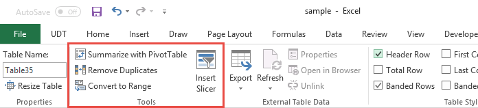
Tools: The following options are available:
- Summarize with Pivot Table: Using Excel data, this creates a pivot table.
- Remove Duplicates: Our article about data cleansing detailed how to remove duplicates quickly.
- Convert to Range: With this option, we can convert an Excel Table into a regular range.
- Insert Slicer (only in Excel 2013 and 2016): Slicer can be familiar with our Pivot tables subject. Its function is similar here. Very useful in filtering and arranging data using a single click.
External Table Data
This menu exports and refreshes data.
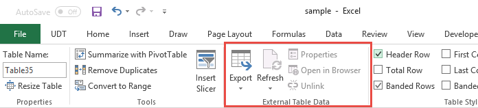
Table Style Options
These are design elements. There are more variants to customize the created table.
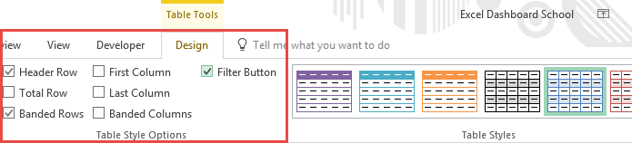
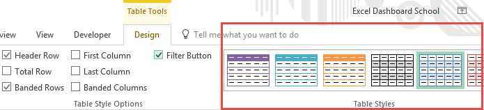
Table Styles
When we don’t have the time to create personal styles, we have many pre-defined themes. The variety is wide; everyone can find the perfect one. We can also create our style by selecting the “New Table Style” option. It is the fastest method if you want to highlight every other row.
Conclusion
Using an Excel Table allows us to structure our data appropriately. Further work is very simple with it. Its biggest advantage is that we can easily expand the original list/range without additional calculations. We recommend its use.
Additional resources: