
Learn how to create a sales dashboard in Excel. The goal is to show the main metrics and provide a comparative view of other products.
Measuring performance and creating a report is not always straightforward. First, we’ll apply the OFFSET function and conditional formatting. This spreadsheet allows the user to select the data dimension and shows sales efficiency immediately.
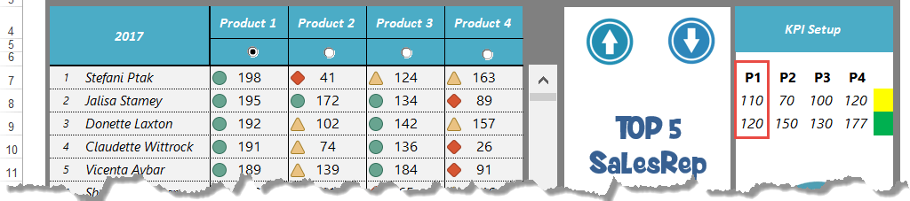
The result looks like this:
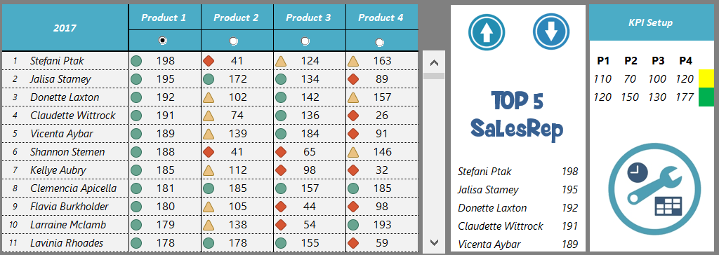
The OFFSET function helps to determine the ranking and grouping as soon as possible, and with the help of formatting, we can analyze the high and low differences. We should rank the highest and weakest performing products to determine which products fail to boom with your customers.
Steps to Create a Sales Dashboard
We’ll use form controls and formulas to make the sales dashboard interactive.
#1. Prepare data
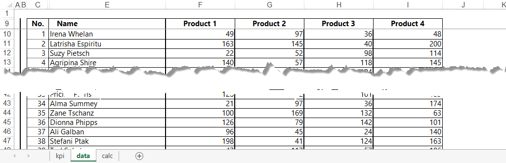
We have the raw data for 100 sales reps and four products. The data looks as shown below.
#2. Create named ranges
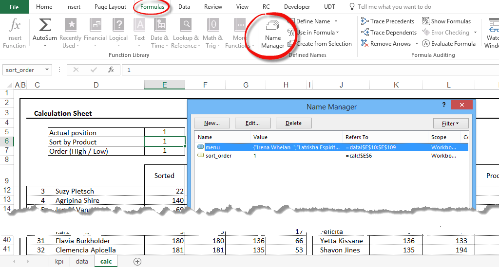
First, create named ranges for further calculations. Next, select the cell or range. In this example, we’ll use both of them. Finally, choose the =data!$E$10:$E$109, the range on the ‘Data’ sheet.
Go to the Formulas tab! In the Defined Names group, click Define Name. Enter a Name (menu) for the range. Select cell E6 and add a name (sort_order). See the results in the picture below!
#3. Use the OFFSET function
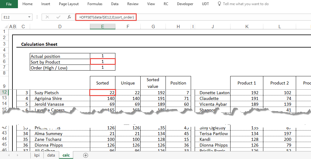
Use the OFFSET function to build a dynamic named range for further calculations. On the calculations sheet, type:
=OFFSET(data!$E10;0;sort_order)
Explanation: How do you get the correct name from the unsorted list? OFFSET(name of the sales rep from data table; 0 = same row; 1st position)
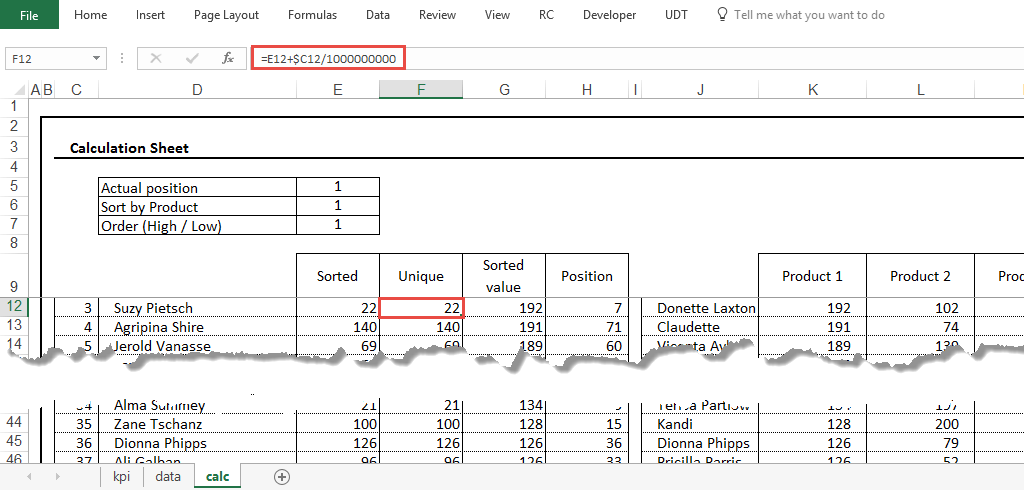
#4. Create a unique list
Use the =E10+$C10/1000000000 formula to create a unique list!
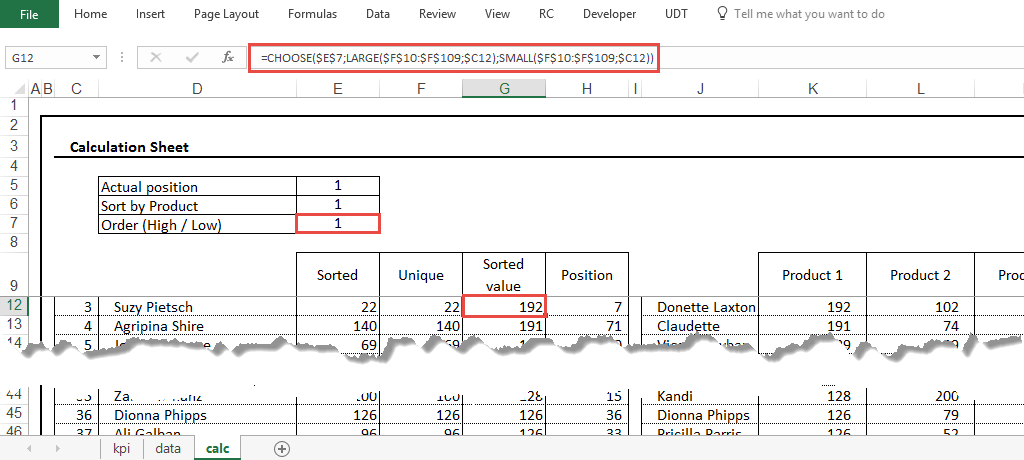
#5. Retrieve the position using the CHOOSE function
Use the CHOOSE, LARGE, and SMALL functions to get the proper value in a range.
=CHOOSE($E$7;LARGE($F$10:$F$109;$C10);SMALL($F$10:$F$109;$C10))
The CHOOSE formula returns a value from a list using a given position or index. For example, CHOOSE(3,” value1″,” value2″,” value3″) returns “value3” since value3 is the 3rd value listed after the index number.
The LARGE function retrieves numeric values based on their position in a list when sorted by value. When sorted by value, the SMALL function retrieves numeric values based on their place in a list.
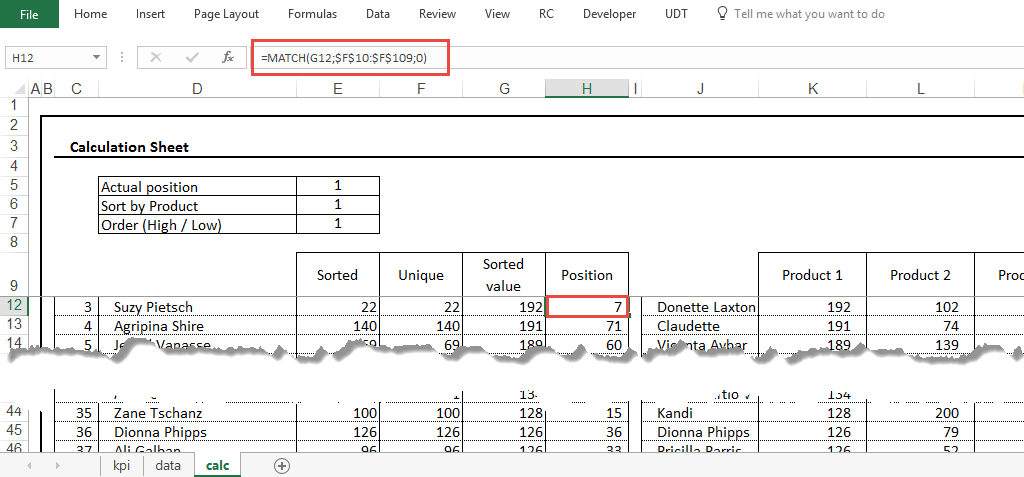
#6. Get the item’s position in an array
To get the position of an item in an array, apply the MATCH function.
=MATCH(G10;$F$10:$F$109;0)
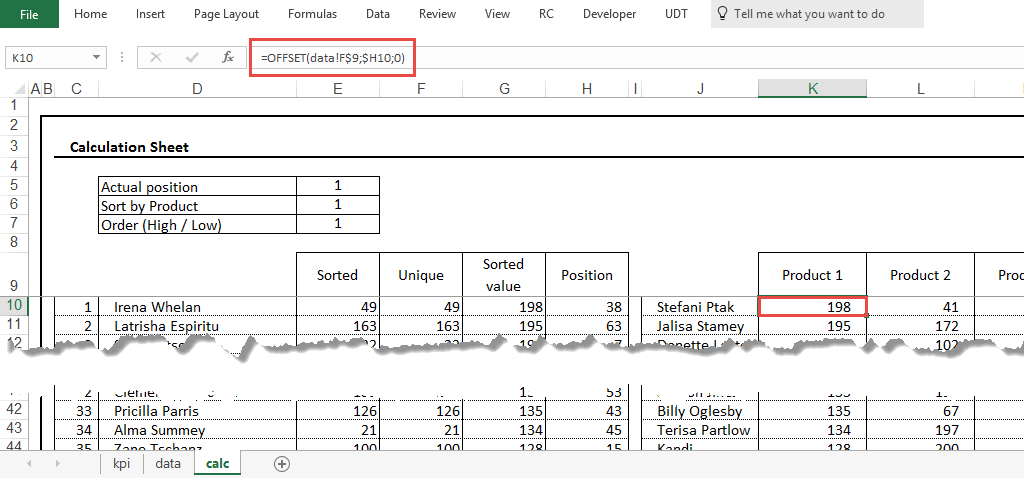
#7. Calculate the 1st position
Now use the OFFSET(data!F$9;$H10;0) to calculate the 1st position for Product 1.
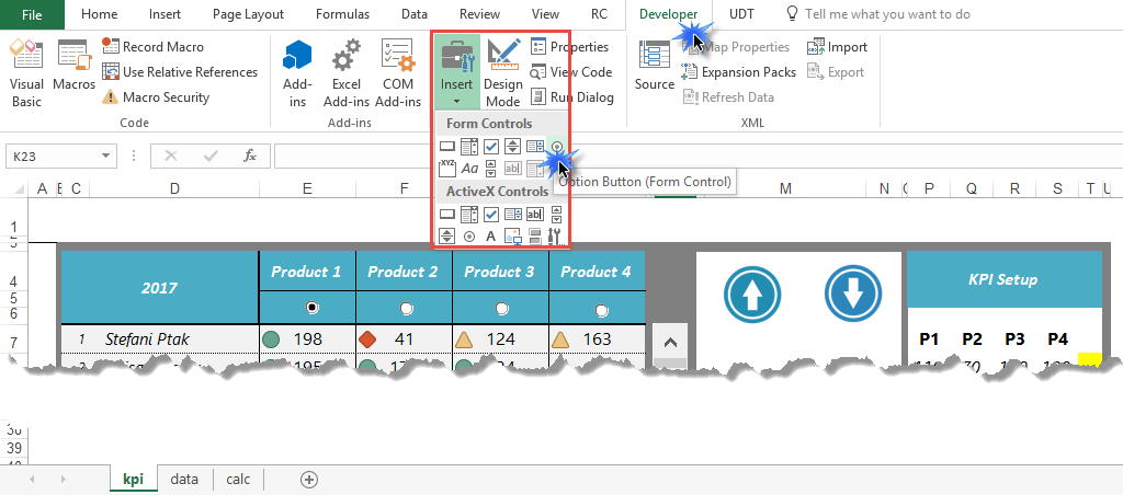
#8. Insert an option button
Insert an option button to make data entry easier. Option buttons are perfect when you have just one choice. To add the Options button, click the Developer tab and select Insert. Finally, under Form Controls, click the Options button icon.
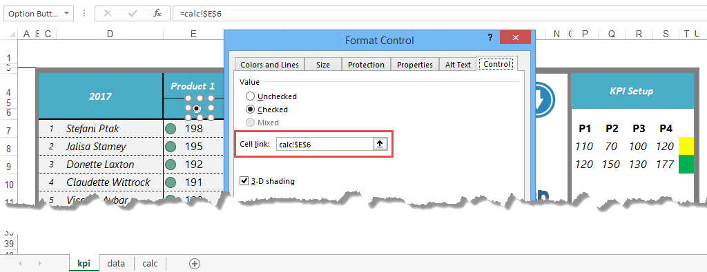
#9. Create a cell link
To add a linked cell, right-click and click on Format Control. Next, jump to the Control tab. Then, enter a cell reference in the Cell link box containing the button’s current state. For example, use the same linked cell (E6 on the calculation sheet) for Product 1 to Product 4.
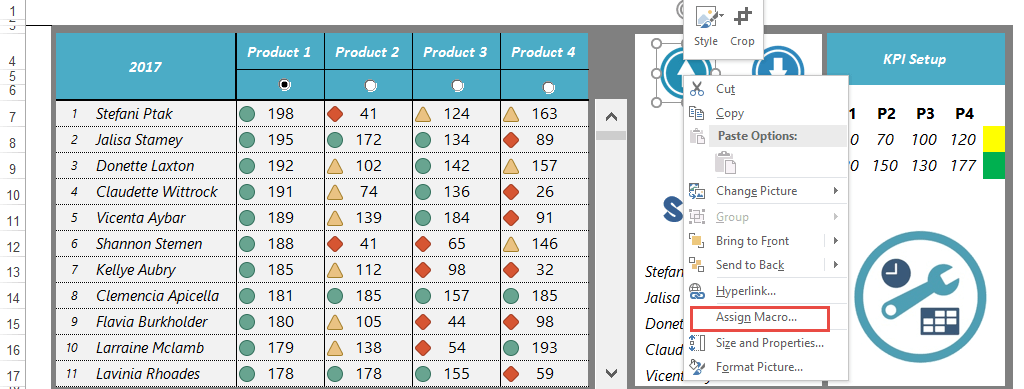
#10. Assign a macro to a picture
To assign a macro to the inserted picture (icon), execute the following steps: Right-click on the image. Next, choose the Assign Macro command. Then, add a macro from the list.
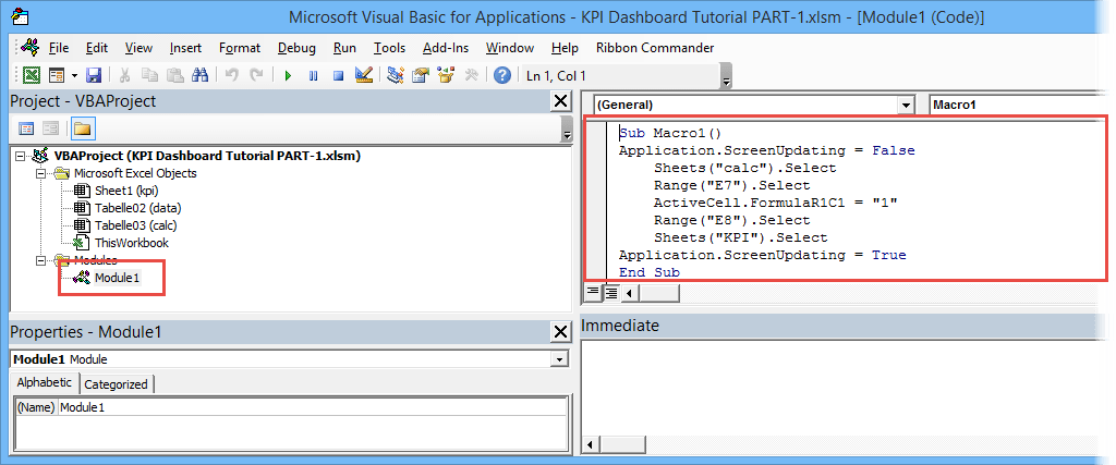
#11. Insert a macro
The macro is very simple. So I think it’s not necessary to explain further.
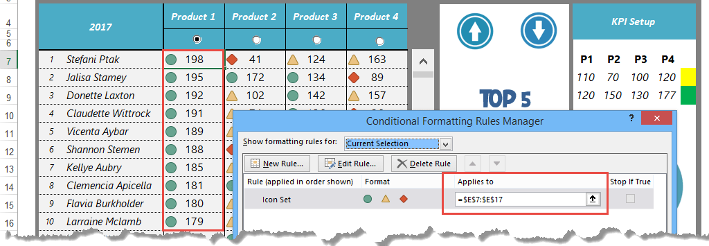
#12. Apply conditional formatting
You can combine the conditional formatting tool with your settings.
#13. Use conditional formatting rules
Use the Conditional Formatting Rules Manager to manage all conditional formatting rules in this worksheet.
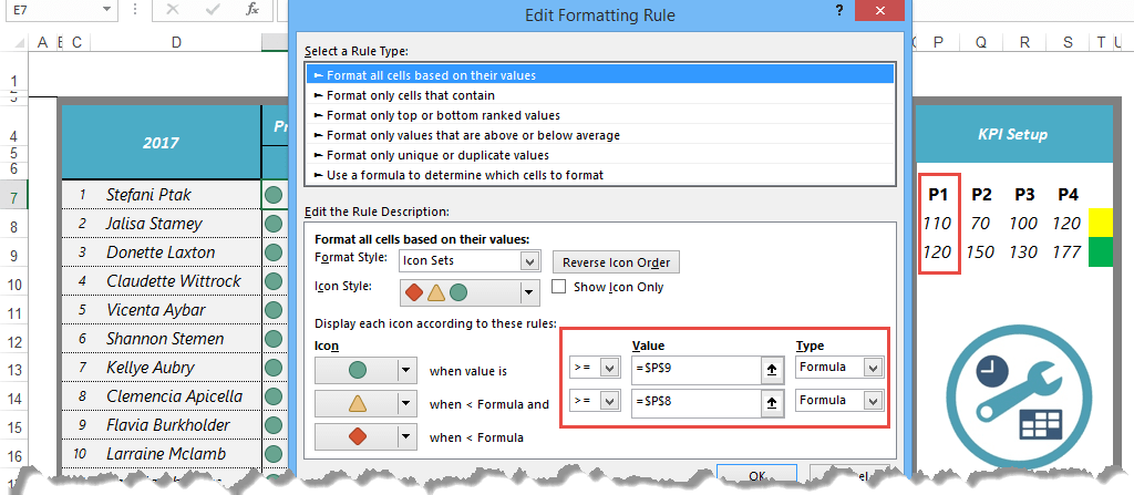
#14. Manage rules
On the Home tab, click Conditional Formatting and click on Manage Rules. Next, select the ‘Format all cells based on their values’ rule type option.
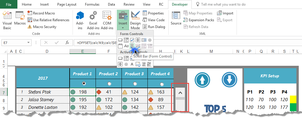
#15. Insert a slider
To insert a slider in Excel, go to Developer Tab –> Insert –> Scroll Bar). Then, click the Scroll Bar button and insert it into the worksheet.
#16. Link the actual value to the slider
Right-click on the Scroll Bar and click on ‘Format Control.’ The Format Control dialogue box will appear. Go to the Control tab and make the following changes to create a scrolling list:
- Current Value: 1
- Minimum Value: 1
- Maximum Value: 76
- Incremental Change: 1
- Page Change: 10
- Cell Link: $E$5 on the calculation sheet.